1. Introduction

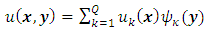
The analysis and design in structural and geotechnical engineering problems requires the calculation of stress and strain which is generally a difficult task because of the uncertainty and spatial variability of the materials’s properties. Various forms of uncertainties arise which depend on the nature of geological formation or construction method, the site investigation, the type and the accuracy of design calculations etc. In recent years there has been considerable interest amongst engineers and researchers in the issues related to quantification of uncertainty as it affects safety, design as well as the cost of projects.

A number of approaches using statistical concepts have been proposed in engineering in the past 25 years or so. These include the Stochastic Finite Element Method (SFEM) [1-3], and the Random Finite Element Method (RFEM) [4-8]. The RFEM involves generating a random field of soil or structure properties with controlled mean, standard deviation and spatial correlation length, which is then mapped onto a finite element mesh. However the number of works on the stochastic stress and strain calculation and their statistical moments are limited. An essential paper on the field is presented by Ghosh & Farhat [9] where the constitutive relation of stress and strain calculated by different approaches.

In the past SFEM has been developed using different expansions of stochastic variables. In this paper we present SFEM [11-13] using the method of Generalized Polynomial

Chaos (GPC) [14]. To descretise the stochastic process of material the Karhunen-Loeve Expansion was used and it is presented. The constitutive relation of stress and strain calculated using the Generalized Polynomial Chaos and verified against Monte Carlo simulation which is treated as the exact solution based on a series of computational experiment.

A numerical example of foundation settlement given in the last part of the paper and the results of settlement compared with those arises from closed form solution. The two methods of stress and strains constitutive relation compared also and the results are presented.

2. Problem Description and Model Formulation

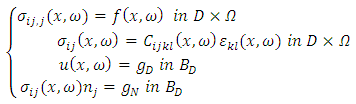
Let us consider a general boundary value problem of computation of probable deformation of a body of arbitrary shape having randomly varying material properties caused by the application of a randomly varying load as shown in Fig. 1.

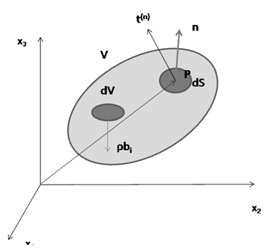Figure 1. Body of arbitrary shape

According to the elasticity theory a boundary value problem can be described as follow:

(1)

And in the weak form as:

(2)

Where:

(3)

(4)

In order to model the problem assuming the sample space where is the σ-algebra and is considered to contain all the information that is available, is the probability measure and the spatial domain of the soil or the structure is . The Elasticity modulus 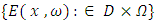and the external load 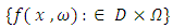considered as second order random fields and their functions are determined and characterized by specific distribution where in our case as lognormal. Considering as and the mean value the standard deviation and the coefficient of variation of Elasticity modulus, the lognormal distribution is given [8]:

(5)

Where the mean values and the variance of the distribution are equal to:

(6)

And

To separate the deterministic part from the stochastic part of the formulation the Karhunen-Loeve expansion has been used. It is considered as the most efficient method for the discretization of a random field, requiring the smallest number of random variables to represent the field within a given level of accuracy. Based on that the stochastic process of Young modulus over the spatial domain with a known mean value and covariance matrix assuming lognormal distribution is given by:

(7)

In practice, calculations were carried out over a finite number of summations (for example 1-5) so the approximate stochastic representation is given by the trancuated part of expansion:

(8)

Where:

are the eingenvalues of the covariance function

are the eingenfunctions of the covariance function

and

The pairs of eingenvalues and eingenfunctions arised by the equation:

(9)

Using the Karhunen-Loeve expansion the stochastic elasticity tensor is given by:

(10)

is expressed in terms of (deterministic) Poisson's ratio as

(11)

To compute the statistical moments of the calculations output we perform a change of variable and [10]. If the random variables are independent and denote the density of then the joint density is given by:

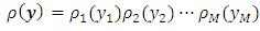(12)

Drakos & Pande [12, 13] developed a new algorithm of Stochastic Finite method using the Generalized Polynomial Chaos (appendix A) and proved that the problem formulation has the final form:

(13)

Where:

(14)

(15)

B is strain displacement matrix.

is the hat function.

is the Polynomial Chaos

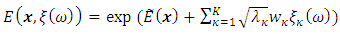
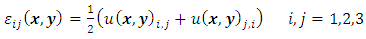
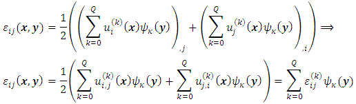
3. Constitutive Relations of Stress and Strain

The calculation of the constitutive relation of stress and strain in the case of stochastic problems is quite complicated especially when the invariant of them are needed where the equations become highly nonlinear. In [9] several numerical integration schemes to evaluate the statistical moments of strains and stresses in a random system is presented. In the current work the propagation of the input uncertainty to the stress and strain relation is modelled by the polynomial Chaos expansion and verified against Monte Carlo simulation which is treated as the exact solution of the problems. 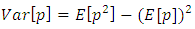The computational implementation of the Monte Carlo Method leads to the random field generation and the requested function gets a new value for each realization. At the end of all simulations the statistical moment are calculated.

The expected value and the variance are given by:

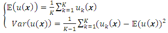(16)

In an elastostatic problem of homogeneous isotropic body one of the field equations that must be satisfied at all interior points of the body is the Strain-Displacement relations:

(17)

Using the displacement polynomial chaos expansion

(18)

Where: Q and ψ are given in appendix A

The equation 17 leads to:

(19)

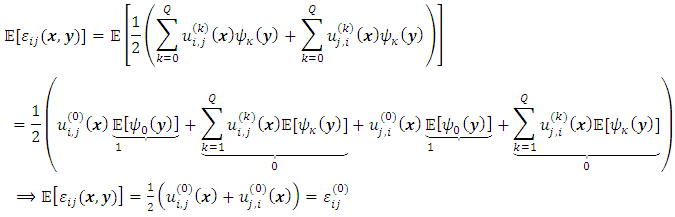
3.1. Expected Value of Strains

According to the polynomial chaos expansion of strains the expected value can be evaluated by the following:

(20)

3.2. Variance of Strains

Respected to the expected value evaluation and the Chaos Polynomial characteristics the variance of the strain tensor can be calculated as:

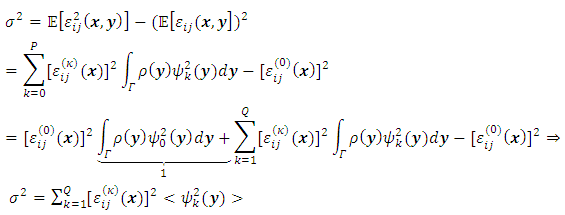(21)

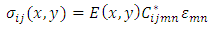
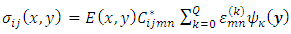
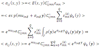
3.3. Expected Value of Stress Tensor

The constitutive relation of stress and strain given by the well known equation of Hooke’s law equation:

(22)

Using the polynomial chaos expansion of strains we get:

(23)

According to the elasticity modulus distribution and the strain tensor Chaos Polynomial expansion the expected value of stress tensor takes the following form:

(24)

3.4. Variance of Stress Tensor

Having calculated the expected value of stress tensor and knowing its stochastic equation of by the Hook’s law constitutive relation, the variance of stress tensor can be calculated as:

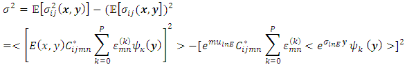Given the elasticity modulus distribution the variance of stress tensor is equal to:

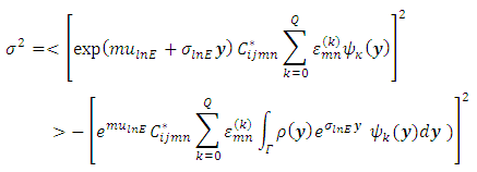(25)

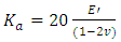
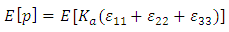
3.5. Pore Pressure Calculation

A major issue in a wide range of geotechnical and geomechanics problem is the estimation of the excess pore pressure in the ground. Using the Chaos Polynomial expansion the statistical moments of pore pressure can be evaluated as following. The pore pressure is given by the following equation:

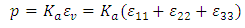(25)

Where:

is the volumetric strain

is shown [15] as

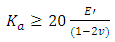(26)

Assuming a minimum value of

3.5.1. Expected Value of Pore Pressure

The expected value of pore pressure is the result of the summation of the expected value of the strain’s Chaos expansion multiplied by the stochastic fluid modulus:

(27)

Replacing the longnormal distribution o elasticity modulus we get:

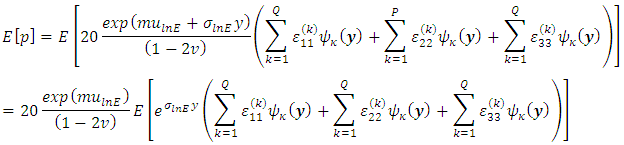And finally

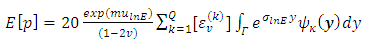(28)

3.5.2. Variance of Pore Pressure

Using the outcome of the pore pressure expected value its variance is given by:

Where:

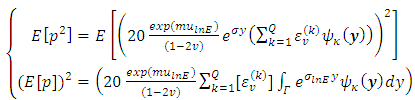(29)

3.6. Invariants of Stress Tensor

It is well known that to solve engineering problem the model itself should be defined independent of the coordinate system attached to the material. Thus, it is necessary to define the model in terms of stress invariants which are, by definition, independent of the coordinate system selected. The physical content of a stress tensor is reflected exclusively in the stress invariants .

Where:

(30)

(31)

(32)

Solving a stochastic problem the statistical moments of stress invariants are needed. In the following paragraphs the calculation of the expected and variance value of each of invariants are presented.

3.6.1. Expected value of I₁

According to the linearity of the excepted value of can be calculated:

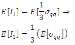Where:

(33)

and

(34)

3.6.2. Variance of I₁

Knowing the mean value of the variance is:

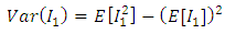But due to linearity:

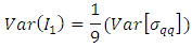Where:

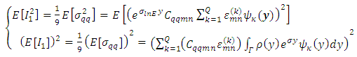(35)

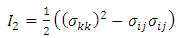
3.6.3. Expected Value of I₂

As shown before:

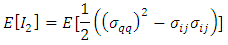This gives

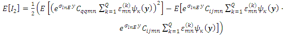(36)

3.6.4. Variance of I₂

The variance of due to the stress product on its equation become highly nonlinear. Thus

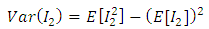Where:

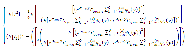(37)

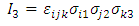
3.6.5. Expected Value of I₃

The high non linearity presented also in the statistical moments of .

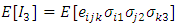This leads to:

(38)

3.6.6. Variance of I₃

Similarly as documented above the variance of is equal to:

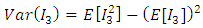Where:

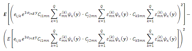(39)

4. Numerical Example

A shallow foundation problem for various values of variation’s coefficient is solved taken to account the randomness of the ground. To estimate the statistical moments of the soil deformation the numerical algorithm of SFEM using the Generalized Polynomial Chaos as described in the previous paragraphs is applied and the results are compared to those obtained by the closed form solution. To avoid the negative values of the elastic modulus assumed to have lognormal. It is known that the settlement beneath a foundation with uniform but random elastic modulus is given by the equation [8]:

(40)

Where: is the deterministic value of settlement with everywhere.

Assuming lognormal distribution for the settlements the mean values is equal to

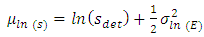(41)

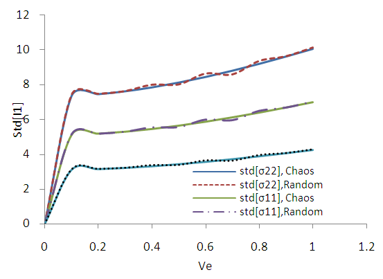
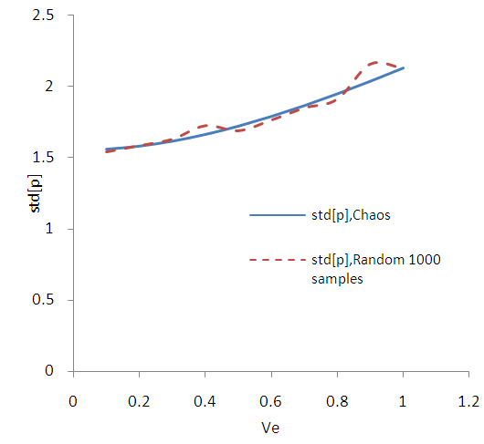
The geometry of the finite elements used for the simulation of the problem presented in Fig. 2. The input data of the problem is the random field modulus with a constant average value equal to 100 Mpa and a fixed Poisson ratio equal to 0.25. Calculations have been made for ten different coefficients of the elastic modulus with a minimum value of 0.1 and then with step 0.1 to a maximum value equal to 1. The randomness of Elasticity modulus in Fig. 3 is shown. For SFEM one dimensional Hermite GPC with order 5 [14] were used. In the Fig. B1 the results of SFEM method comparatively with the closed form solution are shown and they present great accuracy. It is observed that for of v_e = 0.5 the error is equal to 0.8%. In the figures B2-B13 the strains and stress components, the pore pressure and the stress tensor invariants are presented as resulted by the Chaos Polynomial expansion and compared with those raised by the Monte Carlo Method. Simulations of 1000-5000 samples were carried and the convergence of the outcomes decreases as the number of Monte Carlo simulations increases.

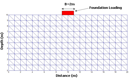Figure 2. Finite element mesh

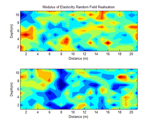Figure 3. Modulus of Random Elasticity of two different realizations

5. Conclusions

To propagate the uncertainties of input parameters to constitutive relations of strain and stress where arises due to spatial variability of mechanical parameters of soil/rock in geotechnical and geomechanics problems, a procedure of conducting a Stochastic Finite Element Analysis has been presented.

An algorithm of Stochastic Finite Element using Polynomial Chaos has been developed. An analysis of settlement of a plane strain strip load on an elastic foundation has been given as an example of the proposed approach. It is shown that the results of SFEM using polynomial chaos compare well with those obtained from closed form solution.

The stress and strain constitutive relation the pore pressure and the stress invariants are modeled by the polynomial Chaos expansion and verified against Monte Carlo simulation which is treated as the exact solution of the problems. The main advantage in using the proposed methodology is that a large number of realizations which have to be made for (Random Finite Element Method) avoided, thus making the procedure viable for realistic practical problems.

Appendix A

Galerkin approximation and Generalized Polynomial of chaos

In order to solve the problem 1 we have to create the new space For that reason the subspace is considered as [10].

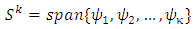(A.1)

Using the dyadic product of the space the space created. Thus

(A.2)

The space has dimension QN and regards the test function v. In the case where exists finite element supported by boundaries condition then the subspace of solution belongs is:

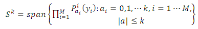
(A.3)

Assuming that the represents a space of univariate orthonormal polynomial of variable with order k or lower and:

(A.4)

The tensor product of the M subspace results the space of the Generalized Polynomial Chaos:

(A.5)

And using (A4)

(A.6)

Where

And

(A.7)

Xiu & Karniadakis [14] show the application of the method for different kind of orthonormal polynomials and in the current paper the Hermite polynomial was used with the following characteristics:

(A.8)

Where:

are the normalization factors, is the  Kronecker delta

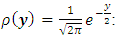is the density function and

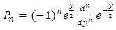(A.9)

For a 3^rd order of one dimension of uncertainty the Hermite Polynomial Chaos is given by:

Appendix B

Results of Numerical Example

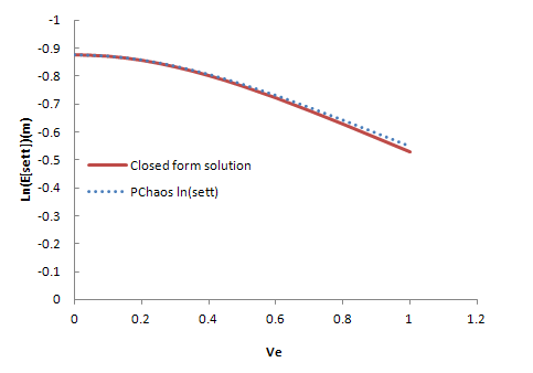Figure B1. Closed form solution and SFEM results

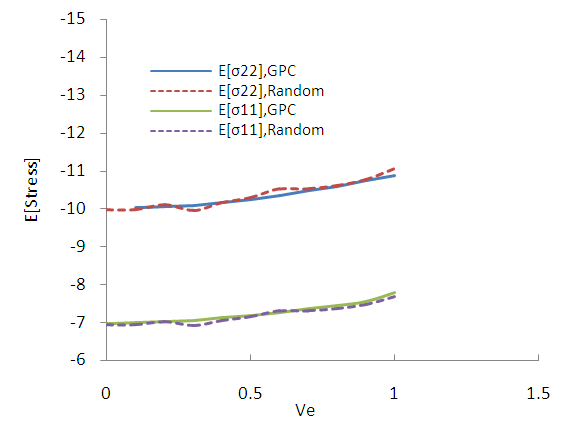Figure B2. Expected value of stress tensor complements (MC 1000 samples)

Figure B3. Standard deviation of stress tensor complements. (MC 1000 samples)

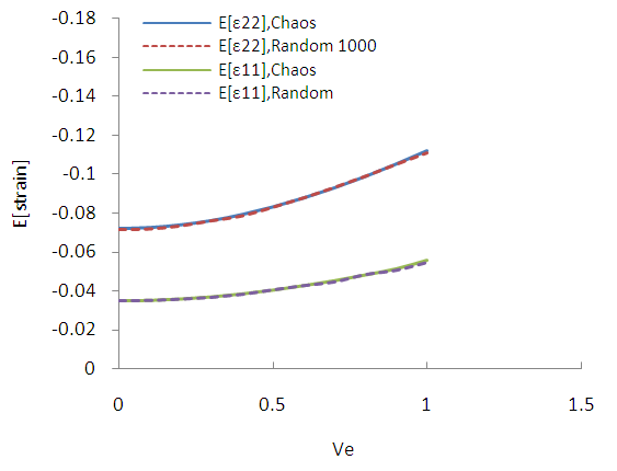Figure B4. Expected value of strain tensor complements. (MC 1000 samples)

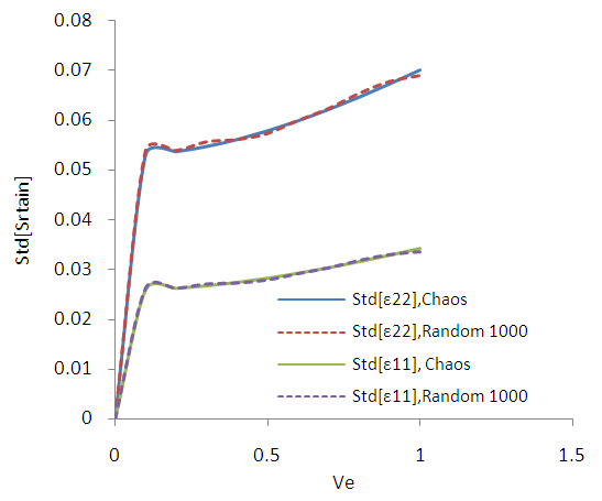Figure B5. Standard deviation of strain tensor complements. (MC 1000 samples)

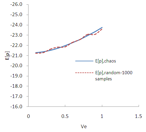Figure B6. Expected value of pore pressure. (MC 1000 samples)

Figure B7. Standard deviation of pore pressure. (MC 1000 samples)

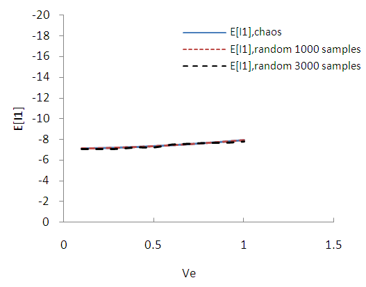Figure B8. Expected value of stress tensor invariant I1. (MC 1000, 3000 samples)

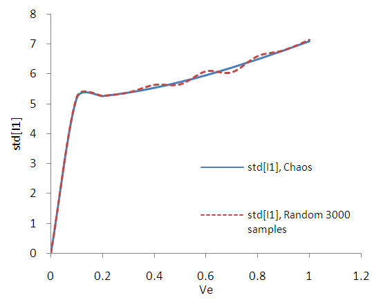Figure B9. Standard deviation of stress tensor invariant I1. (MC 3000 samples)

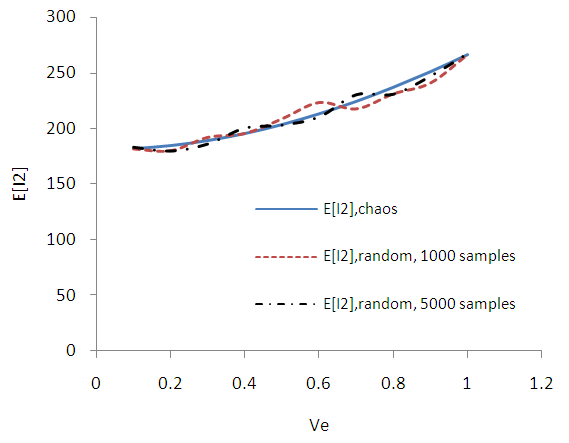Figure B10. Expected value of stress tensor invariant I2. (MC 1000, 5000 samples)

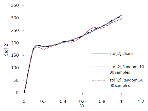Figure B11. Standard deviation of stress tensor invariant I2. (MC 1000, 5000 samples)

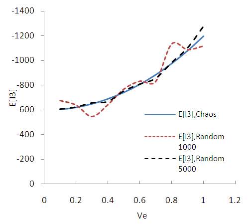Figure B12. Expected value of stress tensor invariant I3. (MC 1000, 5000 samples)

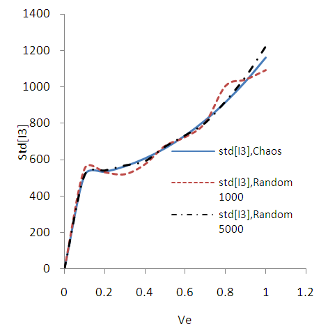Figure B13. Standard deviation of stress tensor invariant I3. (MC 1000, 5000 samples)