Adugna Fita
Department of Applied mathematics, Adama science and Technology University, Adama, Ethiopia
Correspondence to: Adugna Fita, Department of Applied mathematics, Adama science and Technology University, Adama, Ethiopia.
| Email: |  |
Copyright © 2015 Scientific & Academic Publishing. All Rights Reserved.
Abstract
Due to the complexity of many real-world optimization problems, better optimization algorithms are always needed. Complex optimization problems that cannot be solved using classical approaches require efficient search metaheuristics to find optimal solutions. Recently, metaheuristic global optimization algorithms becomes a popular choice and more practical for solving complex and loosely defined problems, which are otherwise difficult to solve by traditional methods. This is due to their nature that implies discontinuities of the search space, non differentiability of the objective functions and initial feasible solutions. But metaheuristic global optimization algorithms are less susceptible to discontinuity and differentiability and also bad proposals of initial feasible solution do not affect the end solution. Thus, an initial feasible solution gauss for gradient based optimization algorithms can be generated with well known population based metaheuristic Genetic Algorithm. The continuous genetic algorithm will easily couple to gradient based optimization, since gradient based optimizers use continuous variables. Therefore, Instead of starting with initial guess, random starting with genetic algorithm finds the region of the optimum value, and then gradient based optimizer takes over to find the global optimum. In this paper the hybrid of metaheuristic global search, followed with gradient based optimization methods shows great improvements on optimal solution than using separately.
Keywords:
Chromosome, Crossover, Gradient, Metaheuristics, Mutation, Optimization, Population, Ranking, Genetic Algorithms, Selection, Subgradient
Cite this paper: Adugna Fita, Metaheuristic Start for Gradient based Optimization Algorithms, American Journal of Computational and Applied Mathematics , Vol. 5 No. 3, 2015, pp. 88-99. doi: 10.5923/j.ajcam.20150503.03.
1. Introduction and Backgrounds
Optimization plays an important role in engineering designs, agricultural sciences, management sciences, manufacturing systems, economics, physical sciences, pattern recognition and other such related fields. The objective of optimization is to seek values for a set of parameters that maximize or minimize objective functions subject to certain constraints. A choice of values for the set of parameters that satisfy all constraints is called a feasible solution. Feasible solutions with objective function value(s) as good as the values of any other feasible solutions are called optimal solutions. In order to use optimization successfully, we must first determine an objective through which we can measure the performance of the system under study. That objective could be time, cost, weight, potential energy or any combination of quantities that can be expressed by a single variable. The objective relies on certain characteristics of the system, called variable or unknowns.The goal is to find a set of values of the variable that result in the best possible solution to an optimization problem within a reasonable time limit. Normally, the variables are limited or constrained in some way. Following the creation of the optimization model, the next task is to choose a proper algorithm to solve it. The optimization algorithms come from different areas and are inspired by different techniques. But they all share some common characteristics.They all begin with an initial guess of the optimal values of the variables and generate a sequence of improved estimates until they converge to a solution. The strategy used to move from one potential solution to the next is what distinguishes one algorithm from another. For instance, some of them use gradient based information and other similar methods such as second derivatives of these functions to lead the search toward more promising areas of the design domain, whereas others use accumulated information gathered at previous iterations. Therefore, in view of the practical utility of optimization problems there is a need for efficient and robust computational algorithms, which can numerically solve on computers the mathematical models of medium as well as large size optimization problem arising in different fields.Now we can formulate our decision making problems as optimization problem of maximization or minimization of single-objective function as: where
where  and
and  comprise the dimensions of the search space
  . A maximization problem can be transformed into a minimization problem and vice versa by taking the negative of the objective function. The terms maximization, minimization and optimization, therefore, are used interchangeably throughout this paper.A single-objective optimization problem can be defined as follows [1].Given
  where
where  and n is the dimension of the search space
  find
find  such that
 and
and 
 | (1.1) |
Subject to  | (1.2) |
Here the vector  is the optimization variable of the problem, the function
  is the objective function, the functions
  are the constraint functions, and vector
  is the global optimal solution of
  .Of course, an equality constraint
  can be embedded within two inequalities
  , and hence, it does not appear explicitly in this paper.We call the set of alternatives
  the feasible set of the problem. The space containing the feasible set is said to be a decision space, whereas
  is a local optimal solution of the region
  when
when  where
where 
 . Note that for unconstraint problems
  .Also optimization variable, decision variable and design variable are terms that are used interchangeable. They refer to the vector
  . We also use objective function, fitness function, cost function and goodness interchangeably to refer to
  . Many real-world optimization problems [2] have mixed discrete and continuous design variables. A common approach to the optimization of this kind of problems, when using classic optimization algorithms, is to treat all variables as continuous, locate the optimal solution, and round off the discrete variables to their closest discrete values. The first problem with this approach is a considerable deterioration of the objective function. The second is the inefficiency of the search due to the evaluation of infeasible solutions. These difficulties may be avoided during the execution of the optimization process by taking into account the type of design variables.In the 12th century Sharaf al-Din al-Tusi, in an attempt to find a root of some single dimensional function, developed an early form of Newton’s procedure [3]. Following Newton’s iterative procedure, and starting from a reasonable guess, the root is guaranteed to be found. This root finding method can be transformed to find either a local optimum or the saddle point of a function. Newton’s method requires the objective function to be twice differentiable, and uses first and second derivative information to construct a successive quadratic approximation of the objective function. It is thus known as a second-order model. The Secant method, a well-known extension of Newton’s procedure, does not need the derivatives to be evaluated directly; rather, they are approximated. Quasi-Newton methods generalize the Secant method to multi-dimensional problems where the inverse Hessian matrix of second derivatives is approximated. The Quasi-Newton methods not only require the existence of the gradient, they are also complex to implement [4].Steepest decent which uses the first-order Taylor polynomial, assumes the availability of the first derivatives to construct a local linear approximation of an objective function and is a first-order method. The idea behind the steepest descent method is to move toward the minimum point along the surface of the objective function like water flowing down a hill. In this method the descent direction is the negative of the gradient of the objective function so that the movement is downhill. The gradient is computed at every iteration and then the next point is a fixed step from the present point. Note that this distance moved along the search direction actually changes since the value of the gradient changes. A stopping procedure is needed. There are two separate stopping criteria, either of which may signal that the optimum value has been located. The first test is to see if there is any improvement in the value of the objective function from iteration to iteration. The second test checks to see if the gradient is close to zero. The conjugate gradient method is a simple and effective modification of the optimum steepest descent method. For the optimum steepest descent method, the search directions for consecutive steps are always perpendicular to one another which slows down the process of optimization. This method begins by checking to see if the gradient at the starting point is close to zero. The conjugate gradient method is suitable for strictly convex quadratic objective functions with finite and global convergence property, but it is not expected to work appropriately on multimodal optimization problems. While numerous nonlinear conjugate gradient methods for non-quadratic problems have been developed and extensively researched, they are frequently subject to severely restrictive assumptions for instance their convergence depends on specific properties of the optimization problem, such as Lipschitz continuity of the gradient of the objective function.When dealing with an optimization problem, several challenges arise. The problem at hand may have several local optimal solutions as in the Figure 3 of test function, it may be discontinuous, the optimal solution may appear to change when evaluated at different times as in the Figure 2b, 2c and Figure 4c, 4d, of test functions and the search space may have constraints. The problem may have a numbers of “peaks” search space, making it intractable to try all candidate solutions in turn. The curse of dimensionality [5], a notion coined by Richard Bellman is another obstacle when the dimensions of the optimization problem are large.Unfortunately, classical optimization algorithms are not efficient at coping with demanding real world problems without derivate information. In other words, selection of the initial points for the deterministic optimization methods has a decisive effect on their final results. However, a foresight of appropriate starting points is not always available in practice. One common strategy is to run the deterministic algorithms with random initialization numerous times and retain the best solution as seen in Figure 1b, 1c, 1c, Figure 2b, 2c and Figure 4b, 4c of test functions; however, this can be a time-consuming procedure.Both gradient and direct search methods are generally regarded as local search methods [6], [7]. Nonlinear and complex dependencies that often exist among designed variables in real-world optimization problems contribute to the high number of local optimal solutions. Classical search methods do not live up to the expectations of modern, computationally expensive optimization problems of today. The shortcomings of classical search methods discussed above are partially addressed and remediated by metaheuristics.These are a class of iterative search algorithms that aim to find reasonably good solutions to optimization problems by combining different concepts for balancing exploration (also known as diversification, that is, the ability to explore the search space for new possibilities) and exploitation (also known as intensification, that is, the ability to find better solutions in the neighborhood of good solutions found so far) of the search process [8].General applicability and effectiveness are particular advantages of metaheuristics. An appropriate balance between intensively exploiting areas with high quality solutions and moving to unexplored areas when necessary is the driving force behind the high performance of metaheuristics [9]. Metaheuristics require a large number of function evaluations. They are often characterized as population-based stochastic search routines which assure a high probability of escape from local optimal solutions when compared to gradient-based and direct search algorithms as seen in Figure 2a and Figure 4a. Metaheuristics do not necessarily require a good initial guess of optimal solutions, in contrast to both gradient and direct search methods, where an initial guess is highly important for convergence towards the optimal solution [10].
2. Mathematical Preliminaries
2.1. Elements of Convex Analysis
Definition: Let A be an n × n square matrix then 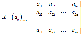 The determinant of A is denoted as |A| or det(A) and defined as
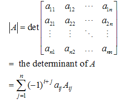 Where:
  the determinant of the matrix
  obtained after deleting
  row and
  column.Definition 2.1: Let A be n × n matrixLet
 Then
Then  is called an eigenvalues of A and
  is called an eigenvector of A. A matrix A will be positive definite if all its eigenvalues are positive; that is, all the values of that satisfy the determinant equation
  should be positive. Similarly, the matrix A will be negative definite if its eigenvalues are negative. A is “positive semi-definite” if all of the eigenvalues are non-negative (≥ 0) and A is “negative semi-definite” if all of the eigenvalues are non-positive (≤ 0)
2.2. Convex Set
Definition 2.2 (algebraic sum of two sets)1. The algebraic sum of two sets is defined as  In case
  is a singleton we use the form
 instead of
  .2. Let
  and
and  . The multiplication of a scalar with a set is given by
  , in particular
 Definition 2.3i. The point
  is said to be a convex combination of two points
  , for some
  ii. The point
  is said to be a convex combination of
  points
  if
if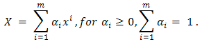 Definition 2.4 A set
  is said to be convex if for any
  and every real number
 , the point
 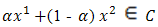 In other words,
  is convex if the convex combination of every pair of points in
  lies in
  .The intersection of all convex sets containing a given subset
  of
of  is called the convex hull of
  and denoted by
  .
.
2.3. Convex Functions
Definition 2.5 A function  is said to be convex if
  is satisfied for all
  and for all
  [0, 1]Moreover, a function
  is said to be strictly convex if for any
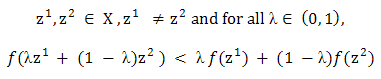 Furthermore,
  is convex if the functions
  are convex for all
  Remark 2.7 If
  is convex, then
  is continuous in
  .
.
2.3.1. Conjugate Function
Definition 2.6 Let  be a convex function
  , then the conjugate (or polar) function of
  is the function
  defined as:
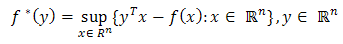 The biconjugate (or bipolar)
 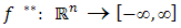 of
of  is the conjugate of
  is defined as:
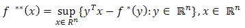 Proposition 2.1 (Fenchel's or Young's Inequality)
 Proof: Follows directly from Definition 2.1.3.1.
2.4. Subgradients of Convex Functions
Definition 2.7 Let  be a convex subset in
  and
and  be a vector valued function.The directional derivative of the function
  at
at  in the direction
  is defined, if it exists, by:
 is said to be Gateaux differentiable at
  if there exists a
  matrix
  such that for any
  ,
,  (x; d) exist
  If
If  is Gateaux differentiable at every
  of
of  , then
  is said to be Gateaux differentiable on
  .Definition 2.1.9 Let
  be a convex function, and let
  . The vector
  is said to be a subgradient of
  at
at  if
if 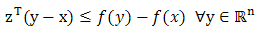 , the set
  is called the subdfferential of at x.Proposition 2.2 Let
  be
be  a convex function from
  to
to  . Then
  The result is a generalization for the condition
  Proof
Proof  is optimal if and only if
  for all x, or equivalently
 for all
  Thus,
Thus,  is optimal if and only if
  Remark 2.3If
  then
then  by conventionIt can be easily established that for convex functions,
  is closed and convex;
 is a singleton if and only if
  is differentiable at x. In this case
  .Proposition 2.3 Let
  be a convex subset in
  and
and  be a vector-valued function. Assume that
  is Gateaux differentiable on
  . Then
  is convex on
  if and only if for every
  ,
,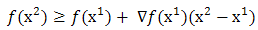 Proof: By definition, if
  is convex, then for all

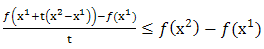 The Proposition holds by taking limit as
  .
.
2.5. Necessary and Sufficient Condition to have Solution
For unconstrained Multivariable optimization the necessary conditionis, if f(x) has an extreme point (maximum or minimum) at  and if the first partial derivatives of f (x) exist at x*, then
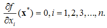 A sufficient condition for a stationary point x* to be an extreme point is that the matrix of second partial derivatives (Hessian matrix) of f (x*) evaluated at x*
 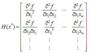 If H is positive definite when x* is a relative minimum point and if H is negative definite when x* is a relative maximum point.
3. Genetic Algorithm
3.1. Introduction
Genetic algorithms is a class of probabilistic optimization algorithms inspired by the biological evolution process uses concepts of “Natural Selection” and “Genetic Inheritance” (Darwin 1859) originally developed by John Holland [11], [12]. Particularly well suited for hard problems where little is known about the underlying search space.The specific mechanics of the algorithms involve the language of microbiology and, in developing new potential solutions, through genetic operations. A population represents a group of potential solution points. A generation represents an algorithmic iteration. A chromosome is comparable to a design point, and a gene is comparable to a component of the design vector. Genetic algorithms are theoretically and empirically proven to provide robust search in complex phases with the above features.Many search techniques required auxiliary information in order to work properly. For e.g. Gradient techniques need derivative in order to chain the current peak and other procedures like greedy technique requires access to most tabular parameters whereas genetic algorithms do not require all these auxiliary information. GA is blind to perform an effective search for better and better structures they only require objective function values associated with the individual strings.A genetic algorithm (or GA) is categorized as global search heuristics used in computing to find true or approximate solutions to optimization problems.
3.2. Initialization of GA with Real Valued Variables
Initially many individual solutions are randomly generated to form an initial population. The population size depends on the nature of the problem, but typically contains several hundreds or thousands of possible solutions. Commonly, the population is generated randomly, covering the entire range of possible solutions (the search space). To begin the GA, we define an initial population of  chromosomes. A matrix represents the population with each row in the matrix being a
  array (chromosome) of continuous values. Given an initial population of
  chromosomes, the full matrix of
  random values is generated by [13]:
 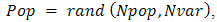 If variables are normalized to have values between 0 and 1, If not the range of values is between
  and
and  , then the unnormalized values are given by:
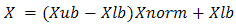 Where
Where  : lowest number in the variable range
  : highest number in the variable range
  : normalized value of variable.But one can generate an initial feasible solution from search space simply as,
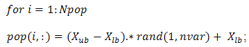 %generate real valued population matrix end; this generates
  population matrix.
3.3. Evaluation (fitness function)
Fitness values are derived from the objective function values through a scaling or ranking function. Note that for multiobjective functions, the fitness of a particular individual is a function of a vector of objective function values. Multiobjective problems are characterized by having no single unique solution, but a family of equally fit solutions with different values of decision variables.Therefore, care should be taken to adopt some mechanism to ensure that the population is able to evolve the set of Pareto optimal solutions.Fitness function measures the goodness of the individual, expressed as the probability that the organism will live another cycle (generation).It is also the basis for the natural selection simulation better solutions have a better chance to be the next generation. In many GA algorithm fitness function is modeled according to the problem, but in this paper we use objective functions as fitness function.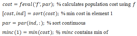
3.4. Parent Selection
During each successive generation, a proportion of the existing population is selected to breed a new generation. Individual solutions are selected through a fitness-based process, where fitter solutions (as measured by a fitness function) are typically more likely to be selected. Certain selection methods rate the fitness of each solution and preferentially select the best solutions. Other methods rate only a random sample of the population, as this process may be very time-consuming.Most functions are stochastic and designed so that a small proportion of less fit solutions are selected. This helps keep the diversity of the population large, preventing premature convergence on poor solutions. Popular and well-studied selection methods include roulette wheel selection and tournament selection and rank based selections [14].
3.4.1. Roulette Wheel Selection
In roulette wheel selection, individuals are given a probability of being selected that is directly proportionate to their fitness. Two individuals are then chosen randomly based on these probabilities and produce offspring.
3.4.2. Tournament-based Selection
For K less than or equal to the number of population, extract K individuals from the population randomly make them play a “tournament”, where the probability for an individual to win is generally proportional to its fitness.
3.5. Reproduction
The next step is to generate a second generation population of solutions from those selected through genetic operators: crossover (also called recombination), and mutation.For each new solution to be produced, a pair of "parent" solutions is selected for breeding from the pool selected previously. By producing a "child" solution using the above methods of crossover and mutation, a new solution is created which typically shares many of the characteristics of its "parents". New parents are selected for each child, and the process continues until a new population of solutions of appropriate size is generated. These processes ultimately result in the next generation population of chromosomes that is different from the initial generation. Generally the average fitness will have increased by this procedure for the population, since only the best organisms from the first generation are selected for breeding, along with a small proportion of less fit solutions, for reasons already mentioned above.
3.5.1. Crossover
The most common type is single point crossover. In single point crossover, you choose a locus at which you swap the remaining alleles from one parent to the other. This is complex and is best understood visually.As you can see, the children take one section of the chromosome from each parent. The point at which the chromosome is broken depends on the randomly selected crossover point. This particular method is called single point crossover because only one crossover point exists. Sometimes only child 1 or child 2 is created, but oftentimes both offspring are created and put into the new population. Crossover does not always occur, however. Sometimes, based on a set probability, no crossover occurs and the parents are copied directly to the new population.
3.5.1.1. Crossover (Real valued recombination)
Recombination produces new individuals in combining the information contained in the parents.The simplest methods choose one or more points in the chromosome to mark as the crossover points [14]. Some of Real valued recombination (crossover) are Discrete recombination, Intermediate recombination and Line recombination Real valued recombination: a method only applicable to real variables (and not binary variables).The variable values of the offspring's are chosen somewhere around and between the variable values of the parents as: where
where 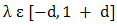 .In intermediate recombination d = 0, for extended intermediate recombination d > 0.A good choice is d = 0.25. (in some literature )Randomly selecting crossover point:
 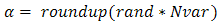 We’ll let
 Where: the m and d subscripts discriminate between the mom and the dad parent. Then the selected variables are combined to form new variables that will appear in the children:
 Where λ is also a random value between 0 and 1, λ=rand The final step is:
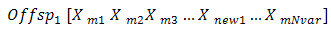

3.5.2. Mutation
After selection and crossover, you now have a new population full of individuals. Some are directly copied, and others are produced by crossover. In order to ensure that the individuals are not all exactly or the same, you allow for a small chance of mutation. You loop through all the alleles of all the individuals, and if that allele is selected for mutation, you can either change it by a small amount or replace it with a new value. The probability of mutation is usually small. Mutation is, however, vital to ensuring genetic diversity within the population. We force the routine to explore other areas of the cost surface by randomly introducing changes, or mutations, in some of the variables. We chose a mutation rate [17],  Randomly choose rows and columns of the variables to be mutated.
 A mutated variable is replaced by a new random number. For Example
 The first random pair is
  .Thus the value in row 5 and column 1 of the population matrix is replaced. By
3.6. Elitism
With crossover and mutation taking place, there is a high risk that the optimum solution could be lost as there is no guarantee that these operators will preserve the fittest string. To counteract this, elitist preservation is used. Elitism is the name of the method that first copies the best chromosome (or few best chromosomes) to the new population. In an elitist model, the best individual from a population is saved before any of these operations take place. Elitism can rapidly increase the performance of GA, because it prevents a loss of the best found solution [15].
3.7. Parameters of Genetic Algorithm
Crossover probability: how often crossover will be performed. If there is no crossover, offspring are exact copies of parents. If there is crossover, offspring are made from parts of both parent’s chromosome. If crossover probability is 100%, then all offspring are made by crossover. If it is 0%, whole new generation is made from exact copies of chromosomes from old population. Crossover is made in hope that new chromosomes will contain good parts of old chromosomes and therefore the new chromosomes will be better [16].Mutation probability: the probability of mutation is normally low because a high mutation rate would destroy fit strings and degenerate the genetic algorithm into a random search. Mutation probability value in some literature is around 0.1% to 0.01% are common. If mutation is performed, one or more parts of a chromosome are changed. If mutation probability is 100%, whole chromosome is changed, if it is 0%, nothing is changed. Mutation generally prevents the GA from falling into local extremes.Population size: how many chromosomes are in population (in one generation). If there are too few chromosomes, GA has few possibilities to perform crossover and only a small part of search space is explored. On the other hand, if there are too many chromosomes, GA slows down. Research shows that after some limit (which depends mainly on encoding and the problem) it is not useful to use very large populations because it does not solve the problem faster than moderate sized populations.
3.8. Termination Conditions
Commonly, the algorithm terminates when either a maximum number of generations has been produced, or a satisfactory fitness level has been reached for the population. If the algorithm has terminated due to a maximum number of generations, a satisfactory solution may or may not have been reached. Thus generational process is repeated until a termination condition has been reached.
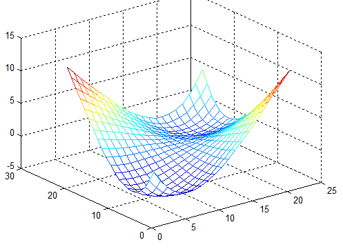
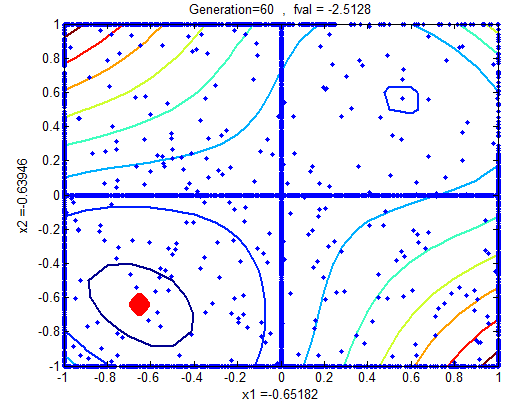
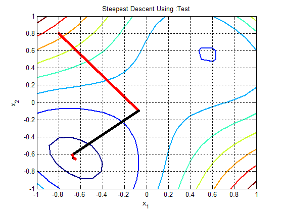
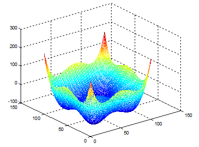
4. Test Functions
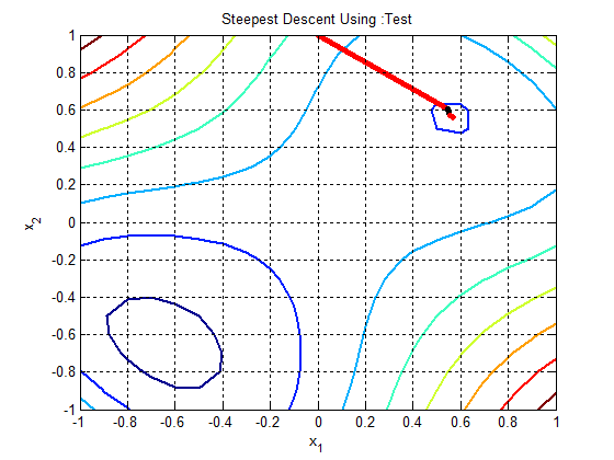
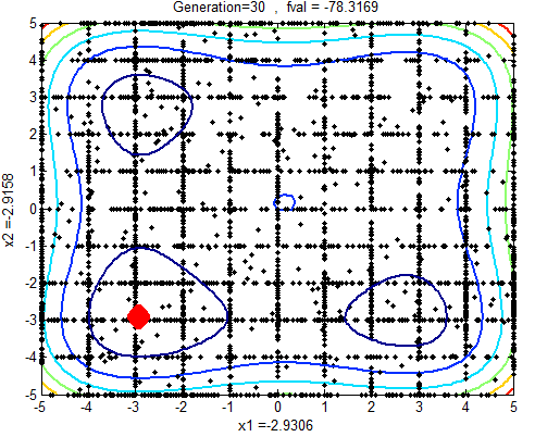
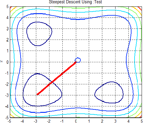
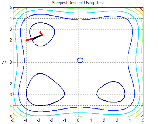
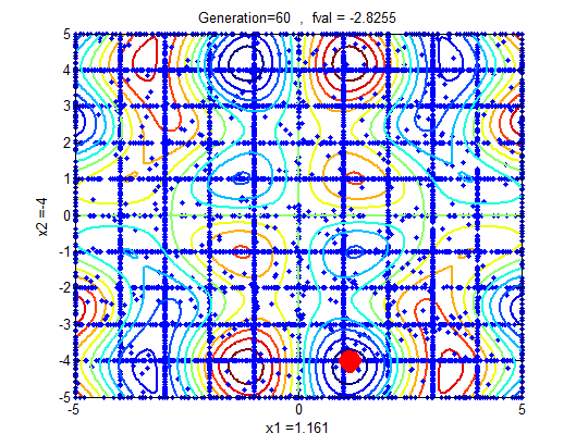
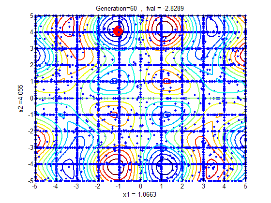
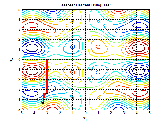
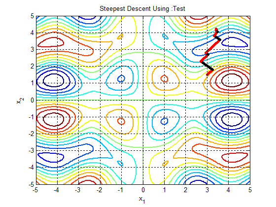
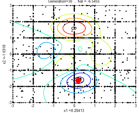
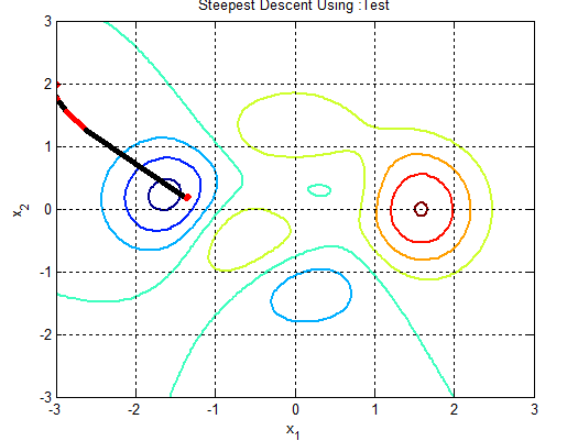
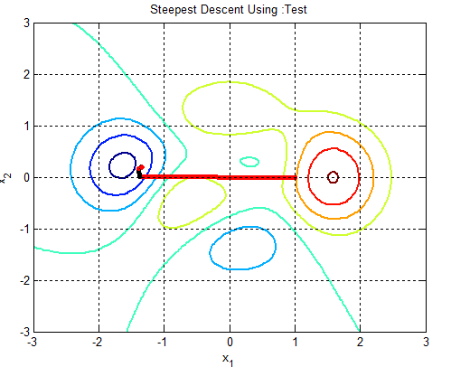
In the following figures the small dots in the case of genetic algorithm is feasible solutions but the red bold dot is optimal solutions, while in the case of the steepest descent the initial and convergence is indicated by zigzag line.
 | Figure 1 |
 | Figure 1a |
 | Figure 1b. 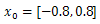 |
 | Figure 1c.  |
 | Figure 1d.  |

 | Figure 2 |
 | Figure 2a |
 | Figure 2b.  |
 | Figure 2c.  |

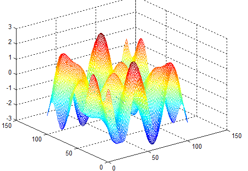 | Figure 3 |
 | Figure 3a |
 | Figure 3b |
 | Figure 3c.  |
 | Figure 3d.  |


 | Figure 4 |
 | Figure 4a |
 | Figure 4b.  |
 | Figure 4c.  |
5. Discussions Using Test Functions
Since the stopping criteria for Genetic algorithm do not grantee optimality and selecting initial feasible solution that converge to global optimal point for gradient based optimization is difficult. Therefore, genetic algorithm iteration followed by gradient based is improving the solution dramatically. Let’s see the iterations of problems 2 and 3 of the test functions.Table 1. Iteration using steepest decent with
 and 8 iterations, Ans = -2.9041, 2.7464, -64.1956 and 8 iterations, Ans = -2.9041, 2.7464, -64.1956 |
| | X1 | X2 | f(x) | | -4.0000 | 2.0000 | -29.0000 | | -3.4396 | 2.1231 | -61.1749 | | -2.7878 | 2.4602 | -62.8970 | | -2.9159 | 2.6993 | -64.1606 | | -2.9019 | 2.7446 | -64.1955 | | -2.9039 | 2.7460 | -64.1956 | | -2.9041 | 2.7465 | -64.1956 | | -2.9041 | 2.7464 | -64.1956 |
|
|
| Table 2. Iteration with Genetic Algorithm last 8 of 10 generations with solution randomly generated form [-5,5], Ans = -2.8978, -3, -78.1656 |
| | X1 | X2 | f(x) | | -3.0000 | -2.8978 | -78.1656 | | -2.9198 | -3.0000 | -78.1615 | | -2.8759 | -3.0000 | -78.1530 | | -3.0000 | -2.8739 | -78.1511 | | -2.8712 | -3.0000 | -78.1482 | | -3.0000 | -2.8708 | -78.1479 | | -3.0000 | -2.8345 | -78.0857 | | -3.0000 | -2.8252 | -78.0627 |
|
|
Table 3. Combinations of the two Iteration using steepest decent with
 obtained from genetic algorithm after 8 iterations, Ans = -2.9041, -2.9039, -78.3323 obtained from genetic algorithm after 8 iterations, Ans = -2.9041, -2.9039, -78.3323 |
| | X1 | X2 | f(x) | | -2.8982 | -3.0000 | -78.1657 | | -2.9037 | -2.9048 | -78.3323 | | -2.9041 | -2.9039 | -78.3323 | | -2.9041 | -2.9039 | -78.3323 | | -2.9041 | -2.9039 | -78.3323 | | -2.9041 | -2.9039 | -78.3323 | | -2.9041 | -2.9039 | -78.3323 | | -2.9041 | -2.9039 | -78.3323 |
|
|
Table 4. Iteration using steepest decent with
 and 14 iterations, Ans = 3.4308, 4.2185, -2.1554 and 14 iterations, Ans = 3.4308, 4.2185, -2.1554 |
| | X1 | X2 | f(x) | | 3.0000 | 1.5000 | -0.8915 | | 3.2551 | 1.7954 | -1.1133 | | 2.6966 | 2.2966 | -1.4361 | | 3.0450 | 2.6913 | -1.6299 | | 2.9321 | 2.7917 | -1.6687 | | 3.6113 | 3.5891 | -1.7856 | | 3.3324 | 3.8261 | -2.0525 | | 3.5021 | 4.0450 | -2.1264 | | 3.4122 | 4.1151 | -2.1477 | | 3.4513 | 4.1678 | -2.1531 | | 3.4262 | 4.1869 | -2.1547 | | 3.4375 | 4.2040 | -2.1552 | | 3.4298 | 4.2086 | -2.1553 | | 3.4327 | 4.2156 | -2.1554 |
|
|
| Table 5. Iteration with Genetic Algorithm last 13 of 20 generations with solution randomly generated form [-5,5], Ans = 1.1541, -4.0000, -2.8254 |
| | X1 | X2 | f(x) | | -1.2481 | 4.0000 | -2.8060 | | -1.0000 | 4.1756 | -2.8060 | | -1.0000 | 4.1381 | -2.8046 | | 1.0000 | -4.1311 | -2.8039 | | 1.0000 | -4.1246 | -2.8030 | | -1.0640 | 4.0000 | -2.8019 | | -1.2619 | 4.0000 | -2.7994 | | 1.0000 | -4.1007 | -2.7987 | | -1.0000 | 4.2370 | -2.7983 | | 1.0000 | -4.0960 | -2.7977 | | 1.0000 | -4.2415 | -2.7973 | | 1.2677 | -4.0000 | -2.7963 | | 1.1541 | -4.0000 | -2.8254 |
|
|
Table 6. Combinations of the two Iteration using steepest decent with
 obtained from genetic algorithm after 5 iterations, Ans = 1.1614,-4.1649, -2.8735 obtained from genetic algorithm after 5 iterations, Ans = 1.1614,-4.1649, -2.8735 |
| | X1 | X2 | f(x) | | 1.1541 | -4.0000 | -2.8254 | | 1.1622 | -4.1632 | -2.8735 | | 1.1614 | -4.1647 | -2.8735 | | 1.1614 | -4.1649 | -2.8735 | | 1.1614 | -4.1649 | -2.8735 |
|
|
6. Conclusions
As many real-world optimization problems become increasingly complex, better optimization algorithms are always needed. Recently, metaheuristic global optimization algorithms becomes a popular choice for solving complex and loosely defined problems, which are otherwise difficult to solve by traditional methods. Gradient and direct search methods are generally regarded as local search methods. Thus, classical methods cannot escape from these local optimal solutions because of the initial gauss for non convex problem. Metaheuristics do not necessarily require a good initial guess, in contrast to both gradient and direct search methods, where an initial guess is highly important for convergence towards the optimal solution.The continuous genetic algorithm will easily couple to gradient based optimization, since gradient based optimizers use continuous variables. Therefore, Instead of starting with initial guess, random starting with genetic algorithm finds the region of the optimum value, and then gradient based optimizer takes over to find the global optimum.In this paper the combination of metaheuristic global search, followed with gradient based optimization methods shows great improvements on optimal solution than using separately.
ACKNOWLEDGMENTS
First of all, I would like to express my deepest and special thanks to Adama Science and Technology University, Department of Applied Mathematics and all members of the department are gratefully acknowledged for their encouragement and support. I would like to extend my thanks to my family for their incredible sup complex port.
References
| [1] | Boyd, S. and Vandenberghe, L. (2004). Convex optimization. Cambridge university press. |
| [2] | Chiong, R., Weise, T., and Michalewicz, Z. (2011). Variants of evolutionary algorithms for real-world applications. Springer. |
| [3] | Soleymani, F. and Sharifi, M. (2011). On a general efficient class of four-step root finding methods. International Journal of Mathematics and Computers in Simulation, 5:181–189. |
| [4] | Broyden, C. (1970). The convergence of a class of double-rank minimization algorithms. IMA Journal of Applied Mathematics, 6(1):76–90. |
| [5] | Bellman, R. (1957). Dynamic Programming. Princeton University Press, Princeton, N.J. |
| [6] | Deb, K. and Goyal, M. (1997). Optimizing engineering designs using a combined genetic search. In Proceedings of the seventh international conference on genetic algorithms, pages 521–528. |
| [7] | Haddad, O., Afshar, A., and Marino, M. (2006). Honey-bees mating optimization (hbmo) algorithm: a new heuristic approach for water resources optimization. Water Resources Management, 20(5):661–680. |
| [8] | Osman, I. and Laporte, G. (1996). Metaheuristics: A bibliography. Annals of Operations Research, 63(5):511–623. |
| [9] | Blum, C. and Roli, A. (2003). Metaheuristics in combinatorial optimization: Overview and conceptual comparison. ACM Computing Surveys (CSUR), 35(3):268–308. |
| [10] | Deb, K. (1999). An introduction to genetic algorithms. In Sadhana (Academy Proceedings in Engineering Sciences), volume 24, pages 293–315. |
| [11] | Holland, J.H. (1975) Adaptation in Natural and Artificial Systems. University of Michigan Press, Ann Arbor. (2nd Edition, MIT Press, 1992.) |
| [12] | Haupt, R.L. (2004) Sue Ellen Haupt: Practical Genetic Algorithms. 2nd Edition, John Wiley & Sons, Inc., Hoboken. |
| [13] | Fita, A. (2014) Three-Objective Programming with Continuous Variable Genetic Algorithm. Applied Mathematics, 5, 3297-3310. http://dx.doi.org/10.4236/am.2014.521307. |
| [14] | Koza, J.R. (1992) Genetic Programming. Massachusetts Institute of Technology, Cambridge. |
| [15] | Ikeda, K., Kita, H. and Kobayashi, S. (2001) Failure of Pareto-Based MOEAs: Does Nondominated Really Mean Near to Optimal. Proceedings of the Congress on Evolutionary Computation, 2, 957-962. |
| [16] | Fita, A. (2014) Multiobjective Programming with Continuous Genetic Algorithm. International Journal of Scientific & Technology Research, 3, 135-149. |
| [17] | http://www.matworks.com |
 Abstract
 Reference
 Full-Text PDF
 Full-text HTML