Ahsan Ali1, Laek Sazzad Andallah2, Zakia Hossain3
1Department of Electronics and Communications Engineering, East West University, Dhaka, Bangladesh
2Department of Mathematics, Jahangirnagar University, Savar, Dhaka, Bangladesh
3Department of Quantitative Sciences, IUBAT-International University of Business Agriculture and Technology, Dhaka, Bangladesh
Correspondence to: Ahsan Ali, Department of Electronics and Communications Engineering, East West University, Dhaka, Bangladesh.
| Email: |  |
Copyright © 2015 Scientific & Academic Publishing. All Rights Reserved.
Abstract
In this paper, a modification of a macroscopic traffic flow model has been presented. In most cases, the source terms that have been appeared in traffic flow equations, represent inflow and outflow in a single-lane highway. So, to demonstrate the effect of inflow, a constant source term has been introduced in a first-order traffic flow equation. Inserting a linear velocity-density relationship, the model is presented. In order to incorporate initial and boundary data, the model is treated as an Initial Boundary Value Problem (IBVP). We describe the derivation of a finite difference scheme of the IBVP which leads to a first order explicit upwind difference scheme. Rigorous well-posedness results and numerical investigations are presented. This paper contains the implementation of the numerical schemes by developing computer programming code and numerical simulation. Numerical schemes are implemented in order to bring out a variety of numerical results and to visualize the significant effects of constant rate inflow.
Keywords:
Macroscopic Traffic Flow Model, Source Term, Explicit Upwind Difference Scheme, Numerical Simulation
Cite this paper: Ahsan Ali, Laek Sazzad Andallah, Zakia Hossain, Numerical Solution of a Fluid Dynamic Traffic Flow Model Associated with a Constant Rate Inflow, American Journal of Computational and Applied Mathematics , Vol. 5 No. 1, 2015, pp. 18-26. doi: 10.5923/j.ajcam.20150501.04.
1. Introduction
As the world’s population grows, traffic management is becoming a mounting challenge for many cities and towns across the globe. Increasing attention has been devoted to the modeling, simulation, and visualization of traffic flows. In an effort to minimize congestion, an accurate method for modeling the flow of traffic is imperative. There is a vast amount of literature on modeling and simulation of traffic flows. Many research groups are involved in dealing with the problem with different kinds of traffic models (like fluid-dynamic models, kinetic models, microscopic models etc.) for several decades. E.g. In [1], the author shows that if the kinematic wave model of freeway traffic flow in its general form is approximated by a particular type of finite difference equation, the finite difference results converge to the kinematic wave solution despite the existence of shocks in the latter. In [2], the author develops a finite difference scheme for a previously reported non-equilibrium traffic flow model. This scheme is an extension of Godunov's scheme to systems. It utilizes the solutions of a series of Riemann problems at cell boundaries to construct approximate solutions of the non-equilibrium traffic flow model under general initial conditions.In [3], the authors consider a mathematical model for fluid dynamic flows on networks which is based on conservation laws. The above discussion motivates us to the study in investigating efficient finite difference scheme to visualize the effect of inflow in a traffic flow simulation.Mainly two approaches generally used in mathematical modelling of traffic flow. One approach, from a microscopic view, studies individual movements of vehicles and interactions between vehicle pairs. This approach considers driving behaviour and vehicle pair dynamics. The other approach studies the macroscopic features of traffic flows such as flow rate  , traffic density
  and travel speed
  . The basic relationship between the three variables is
  . Macroscopic models are more suitable for modelling traffic flow in complex networks since less supporting data and computation are needed. In this paper macroscopic fluid dynamic models are studied both theoretically and numerically. This analysis is mainly focused on the visualization of a constant rate inflow in a single lane highway. The structure of this paper is as follows. In Section 2, we have developed a new model associated with a source term based on the classical LWR model. In Section 3, we derive an exact solution for our model using method of characteristics. In Section 4, based on the study of finite difference method from [4] we formulate explicit upwind difference scheme for the numerical solution of the traffic flow model in a single lane highway. The consequences are presented in Section 5 where different types of numerical experiments show the effectiveness of the constant rate inflow in a single lane highway.
2. Modeling of Vehicular Traffic with Source Term
In the 1950s James Lighthill and Gerald Whitham in [5], and independently Richards in [6], proposed to apply fluid dynamics concepts to traffic flow. In a single road, this traffic flow model is based on the conservation of cars described by the scalar hyperbolic conservation law: | (1) |
where  is the density of cars and
  denote the traffic flow rate (flux) all of which are functions of space,
  and time,
  . Flux
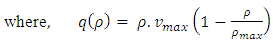
  can be written as the product of the density and of the average velocity
  of the cars, i.e.
  . Inserting this relationship in (1), we obtain
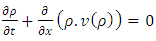 | (2) |
Introducing a source term based on [7] and [11], (2) becomes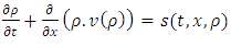 | (3) |
 is the source term denoting inflow or outflow in a particular location of a single lane highway. To avoid complexity of this model, we consider
  is a constant and writing s instead of
 , equation (3) yields:
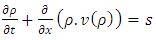 | (4) |
The interpretation and construction of the velocity-density relationship plays a vital role in the macroscopic traffic flow model. The first steady-state speed-density relation is introduced by Greenshields [8], who proposed a linear relationship between speed and density that is as: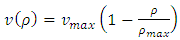 | (5) |
where  is the maximum velocity and
  is the maximum density of the road. Inserting the linear velocity-density closure relationship (5) into (4), we obtain the specific first order non-linear partial differential equation of the form:
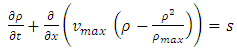 | (6) |
In this paper, we investigate the traffic flow equation given by (6).
3. Analytical Solution of the Model
The non-linear PDE (6) can be solved if we know the traffic density at a given initial time, i.e. if we know the traffic density at a given initial time  , we can predict the traffic density for all future time
  , in principle. Then we have to solve an Initial Value Problem (IVP) of the form:
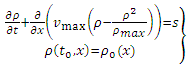 | (7) |
The IVP (7) can be solved by the method of characteristics as follows. The PDE in (7) can be written as: 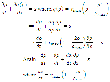 | (8) |
 | (9) |
Integrating (9) we obtain 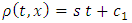 where
where  is the constant of integration. Putting
  and
and  we have
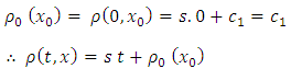 | (10) |
Again by integration from equation (8) we have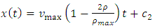 | (11) |
where  is the constant of integration. Putting
  equation (10) becomes
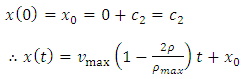 | (12) |
This is the characteristic curve of the IVP (7).Now from (10) and (12) we have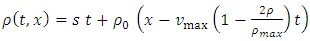 | (13) |
This is the solution of the Cauchy problem (7).However, in reality it is very complicated to approximate the initial density  of the Cauchy problem (7) as a function of t from given initial data, e.g. it may cause a huge error. Moreover, in the case of linear velocity-density relationship it might be such more difficult to solve the IVP by the method of characteristics. Also if we want to employ inflow source term in a particular position, then we can’t describe the effects using (13).Therefore, there is a demand of some efficient numerical methods for solving the traffic flow model (7) as initial value problem.
4. Numerical Solution Using Explicit Upwind Difference Scheme
In order to develop the EUDS (Explicit Upwind Difference Scheme) we consider our specific non-linear traffic model problem as an Initial Boundary Value Problem (IBVP):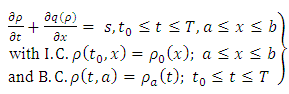 | (14) |
 | (15) |
The IBVP in (14) is well-posed if the characteristic speed  in the range of
  .In order to develop the scheme, we discretize the space and time. We discretize the time derivative
  and space derivative
  in the IBVP (14) at any discrete point
  for
for  and
and . We assume the uniform grid spacing
 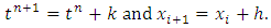 The discretization of
  is obtained by first order forward difference in time and the discretization of
  is obtained by first order backward difference in space. Forward Difference in time:From the Taylor’s series expansion we can write
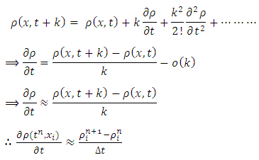 | (16) |
Backward Difference in space:From the Taylor’s series expansion we can write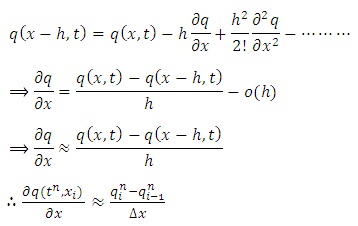 | (17) |
Inserting (16), (17) in (15) and writing  for
for  , the discrete version of the nonlinear PDE formulates the first order explicit upwind difference scheme of the form
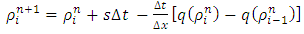 | (18) |
where, 
 | (19) |
In the finite difference scheme, the initial and boundary data and
and  for all
  are the discrete versions of the given initial and boundary values
  and
and  respectively.A stencil is a geometrical arrangement of the nodal group which visualizes the flow of the scheme. The stencil for the explicit upwind difference scheme is presented below:
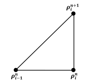 | Figure 1. Stencil of the Explicit Upwind Difference Scheme (EUDS) |
4.1. Stability and Physical Constraint Condition
The implementation of the EUDS scheme is not straight forward. Since vehicles are moving in only one direction, so the characteristic speed  must be positive. Therefore one needs to ensure the well-posedness (physical constraint) condition:
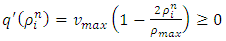 | (20) |
Since the maximum velocity  ,
,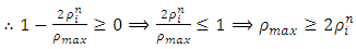 | (21) |
which is the condition for well-posedness.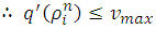 | (22) |
Rewriting the non-linear PDE in (14) as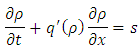 the explicit finite difference scheme (18) takes the form
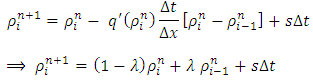 | (23) |
where,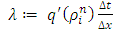 | (24) |
Since we are considering the source term “s” to be a constant, so equation (23) implies that if  then the solution at the new time step is a weighted average of the solution at the old time step. So that this implies
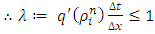 | (25) |
Then condition (25) can be guaranteed via (22) by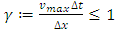 | (26) |
which is the stability condition involving the parameter  .Thus whenever one employs the stability condition (26), the physical constraints condition (21) can be guaranteed immediately by choosing
 | (27) |
4.2. Incorporation of Initial and Boundary Data
In order to perform numerical simulation, we consider the exact solution: | (28) |
We consider the initial condition  , then we have
  | (29) |
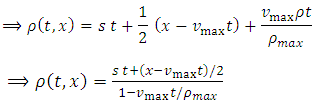 | (30) |
We prescribe the corresponding boundary value by the equation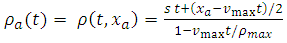 | (31) |
where  denotes the position of the left boundary. To present the numerical solution we avoid the term st from the right hand side of equation (31). Hence the boundary condition takes the following form:
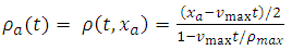 | (32) |
To obtain the density profile we have used the EUDS. In order to use the relevant schemes we have made the following assumptions:• We have considered a highway in a range of 10 (ten) km.• Initially we perform numerical experiment for 6 minutes.• We consider the number of vehicles of various points at a particular time as initial data and constant boundary data.• We have estimated maximum density which is parameterized by  in the traffic flow model. To evaluate
  we have used the following equation
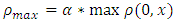 For this we use the initial density for
  and take
 as a constant.Using initial and boundary value on EUDS scheme, we can forecast the traffic flow model.
4.3. Error Estimation of the Numerical Scheme
We compute the relative error in  norm defined by
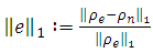 | (33) |
for all time where  is the analytic solution (30) and
  is the numerical solution computed by the explicit upwind difference scheme. Figure 2 shows the relative error remains below 0.001 which is quite acceptable. It also shows a very good feature of convergence of the EUDS scheme.
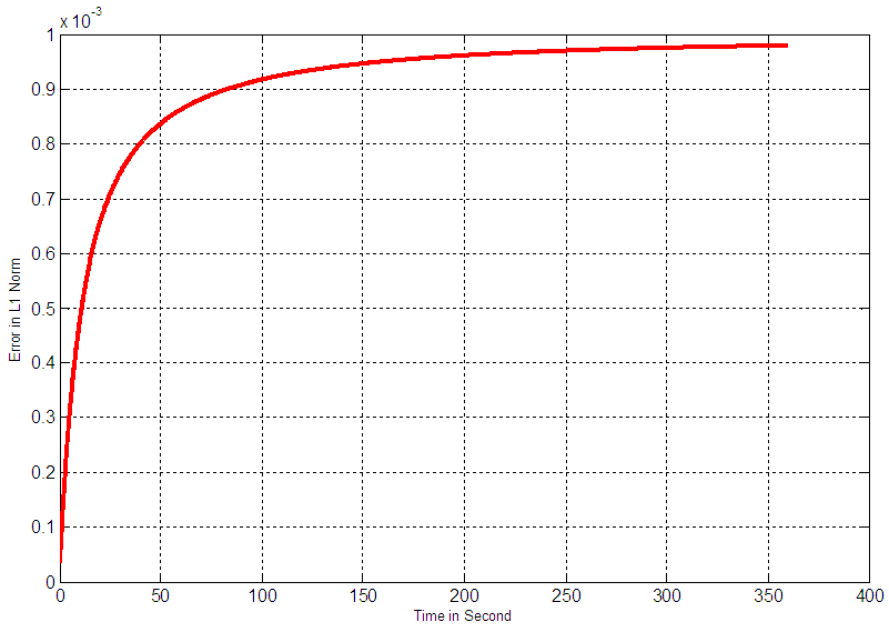 | Figure 2. Convergence of Explicit Upwind Difference Scheme |
5. Numerical Experiments
In this section we present numerical simulation results for some specific cases based on explicit upwind difference scheme (EUDS).
5.1. Density Profile Using EUDS
Initial density profileInitially we consider a highway of 10 kilometers. We choose the maximum velocity of cars is  = 60.12 km/hour. We consider the maximum density
  and we perform numerical experiment for 6 minutes with temporal grid size
  second and spatial grid size
  .We consider the initial condition given by:
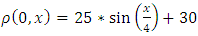 | (34) |
as presented in figure 3 and the constant one sided boundary value for EUDS is 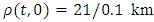 .Initial and 6 minutes density profile for different maximum velocities with an inflow at 5th kmNow we investigate the performance of the EUDS for simulation of a 10 km-freeway with an inflow which is located at 5th km. We consider the initial condition given by equation (34). The constant boundary condition adopted for our numerical simulation is
 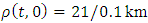 . We consider constant rate inflow s = 5 in the interval [5km, 5.1km].
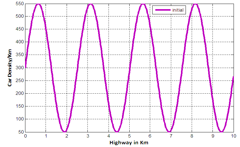 | Figure 3. Initial traffic density for 10 km highway in case of Explicit Upwind Difference Scheme |
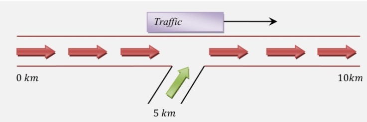 | Figure 4. Layout of a freeway with an inflow |
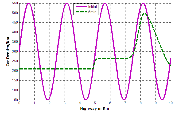
We know that extremely high densities can bring traffic on a roadway to a complete stop and the density at which traffic stops is called the jam density. Figure 5 shows the comparative position of cars between initial and 6 minutes when 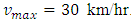 .
.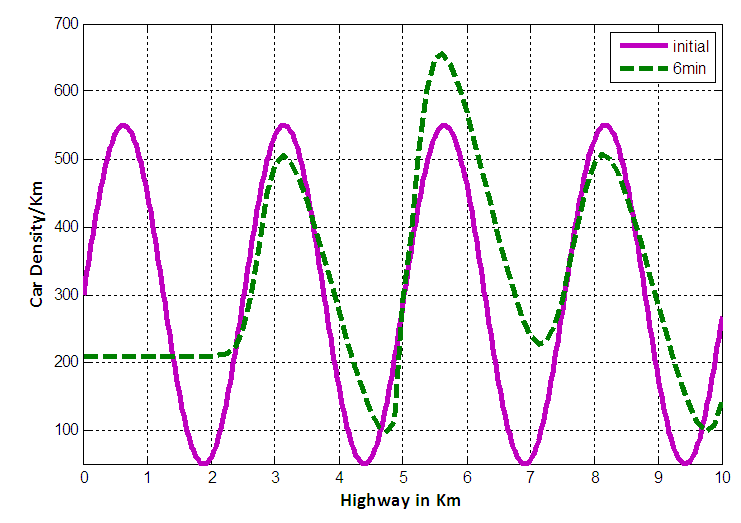 | Figure 5. Comparative position of cars between initial and six minutes in case of EUDS when  |
The curve marked by “dash line” represents the density profile for 6 minutes. Since a constant rate inflow is acting on the 5th km position and the maximum velocity is very low (30km/hr only), so at that point traffic density  exceeds the jam density
  i.e.
i.e.  which leads us to the condition of saturated traffic termed as traffic congestion. Figure 6 and 7 represent the initial position of cars as well as the position after 6 minutes with maximum velocity
 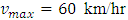 and
and  respectively. We observe that, when
 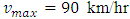 that is in figure 7 the traffic waves are moving faster than the case of figure 6 and 5. In all cases mentioned in this section, we take an inflow source term at 5th km position of our considered 10 km highway where some vehicles enter so that the density of traffic considerably increases at inflow position.
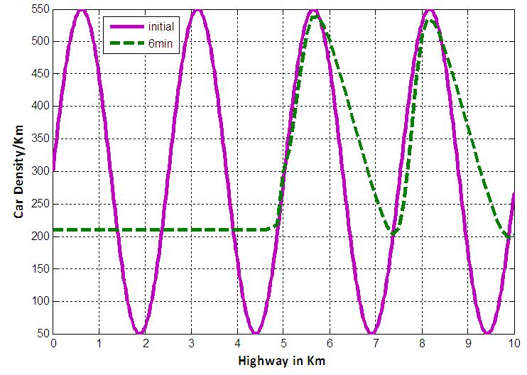 | Figure 6. Comparative position of cars between initial and six minutes in case of EUDS when 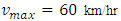 |
 | Figure 7. Comparative position of cars between initial and six minutes in case of EUDS when 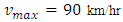 |
5.2. Velocity Profile Using EUDS
The following figures show the velocity profile for car positions at 6 minute with different maximum velocity level consideration. The velocity is computed by the specific linear velocity-density relationship according to Greenshields. This specific relation is of the following form: We consider constant rate inflow
  in the interval [5km, 5.1km].Figure 8, 9 and 10 represent the velocity profile of cars for 6 minute with
  and
and  respectively. According to the behaviour of car velocity marked by “dot-dash line” in the following velocity profile diagrams we see that a constant rate inflow is acting on the 5th km position, so that for high density at that position, the velocity of cars suddenly decreases in all cases.
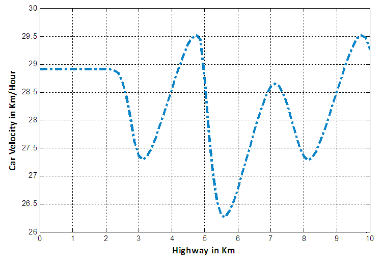 | Figure 8. Velocity profile for car positions at 6th minute in case of EUDS when 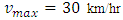 |
 | Figure 9. Velocity profile for car positions at 6th minute in case of EUDS when  |
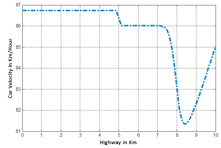 | Figure 10. Velocity profile for car positions at 6th minute in case of EUDS when  |
6. Conclusions
In this paper, a constant source term in the classical LWR model has been introduced to represent constant rate inflow in a single lane highway. Analytical solution for our model based on linear velocity-density relationship has been presented. We have derived explicit upwind difference scheme and for our model. We have also established the stability and physical constraints conditions of these schemes. Finally we have presented numerical results for density and velocity to visualize the effect of constant rate inflow and outflow in a particular position of our considered single lane highway.The significant effect of inflow was visualized by plotting the densities with respect to the distance for various times. We have predicted the velocity with respect to the distance and these results are very much consistent with the values of the parameters as chosen. This motivates us to extend the numerical schemes for further modification of our model.The approach of this research still has some drawbacks which are proposed as topics of our future research.♦ The performance of the model in this paper has been evaluated under limited conditions. The model should be tested with more traffic data collected under various conditions considering even more congestion types, geometric and weather conditions and driver’s efficiency.♦ We have described the analytical solution of our model with initial condition in infinite space. But in reality it is impossible to approximate the initial density for infinite space. It will be our future work to find out the better analytical techniques to solve our model with two sided boundary conditions and initial condition in finite space.♦ In our model, we have discussed the effect of inflow in a single lane highway. For a more detailed simulation of traffic flow for multilane highway, a more differentiated traffic behavior should be considered i.e. the lane changing effects, which we left as our future research work.
References
| [1] | Carlos F. Daganzo. “A finite difference approximation of the kinematic wave model of traffic flow”, Transportation Research Part B: Methodological Volume 29, Issue 4, (Elsevier), p.261- 276, 1995. |
| [2] | H. M. Zhang. “A finite difference approximation of a non-equilibrium traffic flow model”, Transportation Research Part B: Methodological Volume 35, Issue 4, (Elsevier), p. 337-365, 2001. |
| [3] | Gabriella Bretti, Roberto Natalini, Benedetto Piccoli, “A Fluid-Dynamic Traffic Model on Road Networks”, Comput Methods Eng., © CIMNE, Barcelona, Spain 2007. |
| [4] | Randall J. LeVeque, “Numerical methods for conservation laws”, Berlin: Birkhauser, 1992. |
| [5] | Lighthill MJ, Whitham GB (1955) “On kinematic waves. II. A theory of traffic flow on long crowded roads.” Proc Roy Soc Lond Ser A 229:317–345 |
| [6] | Richards PI (1956) “Shock waves on the highway.” Oper res 4:42-51. |
| [7] | Richard Haberman, “Mathematical Models: Mechanical Vibrations, Population Dynamics and Traffic Flow”, Prentice-Hall, Inc., Englewood Cliffs, New Jersey, 1977. |
| [8] | Greenshields, B.D. (1935) “A study of traffic capacity." Highway Research Board 14, 448-477. |
| [9] | Stephen Childress, “Notes on traffic flow”, March 7, 2005. |
| [10] | L. S. Andallah, Shajib Ali, M. O. Gani, M. K. Pandit and J. Akhter, “A Finite Difference Scheme for a Traffic Flow Model based on a Linear Velocity-Density Function”, Jahangirnagar University Journal of Science, Vol. 32, No. 1, pp. 61-71. |
| [11] | Patrizia Bagnerini, Rinaldo M. Colombo, Andrea Corli; “On the Role of Source Terms in Continuum Traffic Flow Models”, Mathematical and Computer Modelling, Volume 44, Issues 9–10, November 2006, Pages 917–930. |
| [12] | S. P. Hoogendoorn, S. Luding, P. H. L. Bovy, M. Schreckberg and D. E. Wolf (Editors), “Traffic and Granular Flow ’03”, Springer. |
| [13] | D. Ngoduy, “Wave propagation solution for higher order macroscopic traffic models in the presence of in-homogeneities”, Institute for Transport Studies, The University of Leeds, University Road 38-42, Leeds LS2 9JT, UK. |
 Abstract
 Reference
 Full-Text PDF
 Full-text HTML