-
Paper Information
- Next Paper
- Paper Submission
-
Journal Information
- About This Journal
- Editorial Board
- Current Issue
- Archive
- Author Guidelines
- Contact Us
American Journal of Computational and Applied Mathematics
p-ISSN: 2165-8935 e-ISSN: 2165-8943
2014; 4(6): 202-217
doi:10.5923/j.ajcam.20140406.04
Generalized Gaussian Elimination (GGE) Solving System of Linear Inequalities or Equalities (LIS-II)
 Abstract
 Reference
 Full-Text PDF
 Full-text HTML
Paul T. R. Wang
Wang Paul_Research, Potomac, Maryland, USA
Correspondence to: Paul T. R. Wang, Wang Paul_Research, Potomac, Maryland, USA.
| Email: |  |
Copyright © 2014 Scientific & Academic Publishing. All Rights Reserved.
The author generalizes the traditional Gaussian Elimination (GE) technique to resolve the feasibility of any system of linear inequalities or equalities. Any linear system consists of either equalities and/or inequalities or mixed of both equalities and inequalities is converted to its homogeneous linear feasibility standard form (HLSF). Variable substitution (VS) in the original Gaussian Elimination is replaced by variable transition (VT) to eliminate a specific variable of choice in a recursive fashion such that at the end only one single variable left to yield the feasible interval for the selected variable if such an interval exists. Note that the feasible interval of a specific variable can be null, single value, bounded below and above, bounded below only, bounded above only, or both unbounded above and below. Furthermore, the feasible interval of a given variable if it exists must also include its integer or binary solution or solutions. It is further shown that the original GE is indeed a special case of the GGE and both GE and GGE share Identical computational complexity that is bounded by the worst case of  . GGE is applicable to any linear system with a finite number of variables, n, and m, a finite number of equalities, inequalities, or mixed constraints. GGE can be used to resolve the feasibility of a given linear system with number of variables and constraints over millions or more. The validity of GGE in dealing very large linear system not only addresses the feasibility of linear systems, it may also resolve the computational complexity of the class of NP-complete (NPC) mystery. This innovative GGE technique is applied to various linear programs with unique solution, unbounded solution, or no solution to illustrate its correctness and applicability. GGE is also shown to be applicable in resolving differential variational inequalities (DVI) for both scientific and engineering applications.
Keywords: Homogenerous Linear Systems, Linear Inequalities, Feasibility, Feasible Interval, Gaussian Elimination, Differential Variation Inequalities, Linear Programs, Computational Complexity
Cite this paper: Paul T. R. Wang, Generalized Gaussian Elimination (GGE) Solving System of Linear Inequalities or Equalities (LIS-II), American Journal of Computational and Applied Mathematics , Vol. 4 No. 6, 2014, pp. 202-217. doi: 10.5923/j.ajcam.20140406.04.
Article Outline
1. Introduction
- Very large system of linear inequalities with thousands or millions of variables and/or constraints are very tough to resolve. Typically, linear inequalities are solved with the famous Simplex method [1-4] the ellipsoid method [6], or the interior points method [7, 11]. Whether or not a linear system is solvable or whether or not a feasible linear system contains integer or binary solution is one of the most challenging questions known as NP-complete (NPC) for applications in operstions research (OR) [10]. In this paper, the author proposes an innovative approach that generalizes the well known Gaussian Elimination (GE) for linear equalities to resolve the feasibility problem of a system of linear inequalities. Instead of variable subsittution, it is replaced by variables transition to eliminate recursively variables of choice until only one single variable is left to determine the feasible intervl associated of the specific variable. The technique is coined as the Generalized Gaussian Elimination (GGE) for linear systems. Furthermore, it is shown that GE is simply a special case of GGE and that both GE and GGE share the same computational complexity. Simple LPs are used to illustrate for all possible cases of feasibble intervals such as single value (unique), infinite many solutions with distinct upper and lower bounds, or both bounded and unbounded cases.
2. Homogeneous Linear Systems Feasibility (HLSF) with New Notations [17-19]
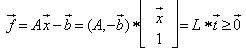
- Given any system of linear inequalities or equalities in vector and matrix form,
 where
where  is an n by m matrix,
  and
and  are m by 1 and n by 1 column vectors respectively.We define the homogeneous linear system feasibility (HLSF) for
  as follows
  where
where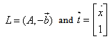 | (1) |
 is referred to as the feasibility vector of the original linear system of inequalities
  .Note that any system or subsystem of linear equalities
  can always be converted into a system or subsystem of linear inequalities as
  .The author adopted the following new notations to simplify the illustration of GGE:Let
  be an 1 by n row vector, and let
 be the 1 by n-1 sub-vector of
  .With such a new notation, it is clear that for the dot product of two vectors
  and
and  we have,
 | (2) |
 , we have
  Given the following homogenous linear inequality (HLI):
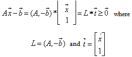 | (3) |
 where
where | (4) |
 to highlight the nonexistence or absence of the variable,
  , from the function (either an equality or an inequality) for
  .
.2.1. A Literature Overview and Motivation
- Traditionally, linear inequalities are resolved as linear programs using either the Simplex methods (Dantzig, 1947), Crisis Cross algorithms (Fukuda & Terlaky, 1997), interior point method (Khachiyan, 1979), projective algorithms (Strang, 1987), path-following algorithms (Gondzio & Terlaky, 1996), and penalty or barrier functions (Nocedal and Wright, 1999). Most approaches centered on iterative searching for feasible points within the n dimensional polytope, i.e., the n-polytope, defined by the constraint linear inequalities. The author with his colleagues [18] proposed a new approach that recursively reduces the worst infeasibility, the sum of all infeasibility, and the number of constraints with the worst infeasibility based upon nonzero coefficients or a subset of the nonzero coefficients that defines the given system of linear inequalities [18]. Such an approach is capable of finding the exact solution if such a feasible solution is unique, a feasible solution if there are more than one solution. For linear system that does not have a feasible solution, this approach is capable of minimizing the sum of all infeasibility or the worst infeasibility, and pinpointing to the relevant coefficients to reveal true conflicts of the linear system [18].Over a five years period from 2009 to 2014 the author presented three new techniques in dealing with linear systems with both equalities and inequalities were propose by the author and his colleagues during the past few years. The first technique (LIS-I) that examines the atomic components of system of linear inequalities is a set of algorithms that recursively reduce the sum of all infeasibility, maximum infeasibility, and the number of constraints with the maximum infeasibility [17, 18], This paper details a generalized Gaussian Elimination (GGE) to obtain the feasible interval of individual variable as LIS-II. A third technique as LS-III utilizes both projective and orthogonal geometry of unit vectors over the surface an n-dimensional hyperspace as the unit-shell and the concepts of equal distanced points to selected set of points on the unit shell with increasing rank recursively to locate a solution if such a solution does exists [19].
3. The Generalized Gaussian Elimination (GGE) Algorithm for HLSF
- Let a HLSF in its standard form as (1)
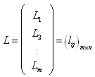
 where the constraint matrix, Let the HLSF
  with n constraints and m variables , then
  , is an n by m+1 matrix with n linear constraints and variables with
 . We have the i-th column of
  ,
,  , and the j-th row of
  ,
,  is respectively:
  and
and  To eliminate a specific variable,
  from
from  , GGE requires the following steps:Step 1: normalization;Step 2: rows permutation by sign;Step 3: sorting of rows by decreasing number of nonzero coefficients;Step 4: replacing rows using binding transition; Steps 1 to 4 are repeatedly applied to eliminate other variables until only the desirable variable left.When only one variable is left, the final HLSF uniquely defines both an upper bound and a lower bound as the feasible interval for remaining variable that is not eliminated.Note that the feasible interval
  with
with may have the following 6 possible cases:(i) no solution such that
  with
with  (ii) unique solution with
  , i.e., we have
  (iii) bounded interval with infinite many solutions as
  such that
  with
with  (iv) bounded above as
  such that
  (v) bounded below as
  such that
  (vi) unbounded above and below as
  such that
  Note: (vi) may not exist; it is listed for completeness.Assume that a selected column variable,
  , is to be eliminated, the detailed description of each step for the GGE is provided as follows:Step 1: Normalization: Normalization of column
  associated with the variable
  is to force all nonzero coefficients of
  has value of 1 for all positive numbers and -1 for all negative numbers and zero otherwise. It is equivalent to construct a diagonal matrix
  where
where  if
if  and
and  if
if  such that
  .Note that Multiplying
  by
by  is simply dividing the k-th row of
  by 1 if
  and the j-th row of
  by
by  if
if  . In other words, we have:
 Note that we have the i-th column of
  is
is  =
=  where
where  if
if  ,
,  if
if  , and
, and  if
if  , for
, for  .Upon the completion of Step 1, the i-th column, associated with the variable,
  consists of only three values, 1, -1, or 0.Step 2 is needed to group rows in
  by the signs in
  in its i-th column and also sort rows in each group by decreasing number of nonzero coefficients (nzc) of the associated row. In equation notations, We are rearranging the rows of
  into three parts by a row permutation matrix,
  , such that
  where
where  and the i-th column of
  is
is  the i-th column of
  =
= , and the i-th column of
  =
= . Furthermore, we haveStep 3. Identifying most and least binding rows: Both
  and
and  are sorted in decreasing order of
  such that
  if
if  where
where  is defined as the number of nonzero coefficients of the r-th row of
  . We refer to rows in
  or
or  with the maximum nzc(r) as binding rows. Two cases of binding rows must be separated properly to locate the least and most binding rows. Let row r in
  be, we have
 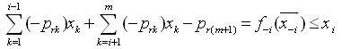 It is possible that another binding row s in
  as:
as: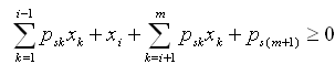 , we have
 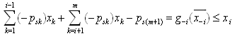 Note that if
 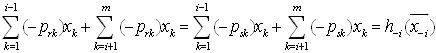 , we have
 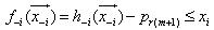 and
and  , hence, the most lower binding (MLB) row for
  is row j such that
  . Similarly, let row r in
  be
be 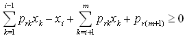 , we have
 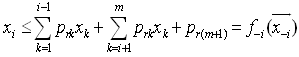 It is possible that another binding row s in
  as:
as: 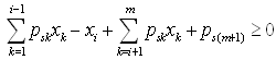 , we have
 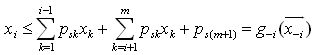 Note that if
 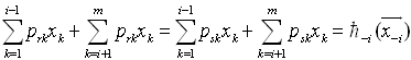 , we have
 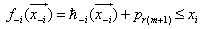 and
and 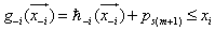 , hence, the least upper binding (LUB) row for
  is row k such that
  .Elimination of the variable
  must preserve the most and/or least binding rows with respect to all the connected variables included and accounted for.Step 4. Note that each row in
  uniquely defines a lower bound of
  with respect to all other variables in
  . Similarly, each row in
  uniquely define an upper bound of
  with respect to all other variables in
  . Select distinct binding rows from
  and
and  such that we have:
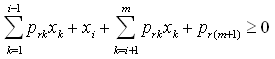 if row r in
  and
and 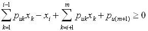 if row u in
  Consequently, we have a lower bound for
  from a binding row in
  as
as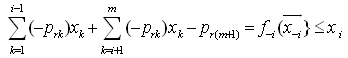 and an upper bound for
  from a binding row in
  as
as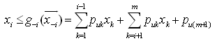 As shown in Step 3, a unique most lower binding (MLB) row and least upper binding (LUB) row for
  may be identified if such binding relationship exists.From this two extreme binding rows, the variable,
  , can be safely and successfully eliminated as:
 For each row
  within
  we have
 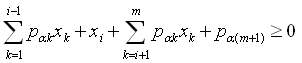 i.e.,
i.e., 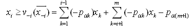 Consequently, we have
  i.e.,
i.e.,  Similarly, for each row
  within
  we have
 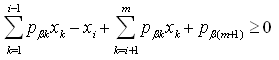 i.e.,
i.e.,  Consequently, we have
  i.e.,
i.e.,  Note that rows in
  do not contain the variable,
  . In other words, we have shown that the variable,
  may be eliminated completely and safely from every row in
  without loss of all the binding inequalities that include all possible lower or upper bounds in terms of the remaining variables,
  Note that steps 1 to 4 may be applied recursively to eliminate any specific ordering of variables in
  such that only a specific variable,
  left such that we have the final inequalities:
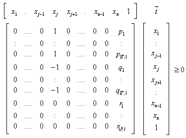 | (5) |
 .In other words, we have:
 where
where  is the number of rows in
  and
and  is the number of rows in
  Let
Let 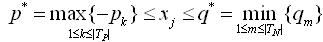 , then
  uniquely defines a feasible interval for the variable,
  . Consequently, we may have the following 6 possible cases for
  .(i) no solution such that
  if
if  (ii) unique solution with
  with
with  i.e., we have
  . (iii) bounded interval with infinite many solutions as
  if
if 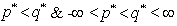 . (iv) bounded above only as
  if
if  .(v) bounded below only as
  if
if  . (vi) unbounded above and below as
  if
if  and
and  .
.4. Examples
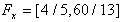
- To illustrate the validity, capability, and correctness of GGE, we provide feasible intervals for simple inequalities computed by GGE that are easily verifiable and sample linear programs covering with unique solution, no solution, or unbounded cases as follows:Example #1
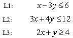 | (6) |
 is:
is: | (7) |
 | (8) |
 Eliminating y, we have the following inequalities
 | (9) |
 Example #2
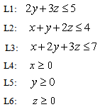 | (10) |
 is:
is: | (11) |
 | Figure 1. Feasible Intervals  and and  |
 | (12) |
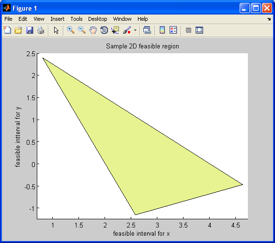
 Eliminating variable x and y with (11), we have the following inequalities:
 | (13) |
 Eliminating variables x and z with (11), we have the following inequalities:
 | (14) |
 Figure 6 illustrates the feasible region for these feasible intervals.
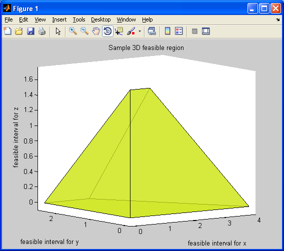 | Figure 6. Feasible Intervals for  , ,  , and , and  |
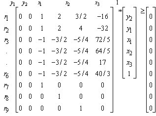
 The self-dual LP as Homogeneous Liner Inequalities (HLI) (Wang, 2013):
 Consider the primal and dual LP pair:
 The corresponding HLFS for this LP as self-dual form [18, 19] is:
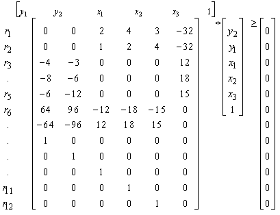 | (15) |
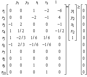
 , normalize column
  we have:
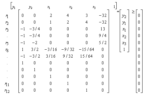 | (16) |
 and MLB
  to eliminate
  , we Have
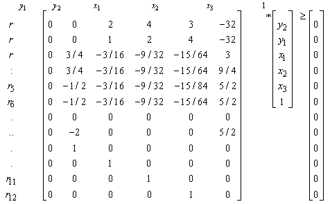 | (17) |
 , we have:
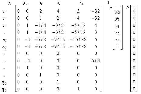 | (18) |
 and LUB
  to eliminate
  , we have
 | (19) |
 | (20) |
 and LUB
  to eliminate
  , we have
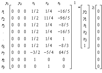 | (21) |
 and the removal of identical rows, we have:
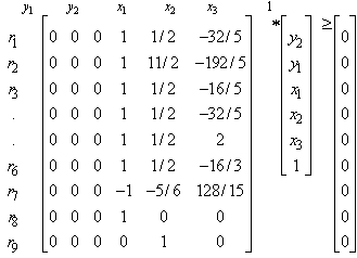 | (22) |
 and LUB
  to eliminate
  , we have
 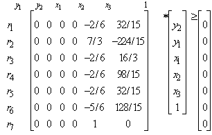 | (23) |
 and the removal of identical rows, we have:
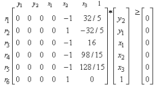 | (24) |
 and the LUB is obtained from row
  such that
  and
and  = 6.4Since MLB=LUB=6.4, we conclude that the variable
  has unique solution with
  From (21) with
  = 6.4, for
  the MLB is
  and LUB =3.2 Hence,
  has unique solution
  = 3.2Substituting
  and
and  = 3.2 into (19), we obtain the MLB and LUB for
  as MLB = 0 and LUB =
  ; Hence,
  has unique solution
  .Substituting
  ,
, = 3.2 and
  = 0 into (17), we obtain the MLB and LUB for
  asMLB =
 and LUB =
 ; Hence,
  has the unique solution = 0.2.Substituting,
 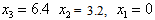 , and
, and  = 0.2 into (15), we obtain the MLB and LUB for
  as MLB =
  and LUB =
  = 2.1; Hence,
  has unique solution
 .Consequently, both the primal and the dual LPs are resolved by applying the GGE algorithm to (15) with the unique optimal solution of
  Example #4 LP with no solutionConsider the LP:
 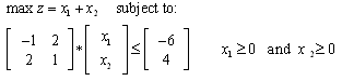 The corresponding HLFS for this LP as self-dual form [19] is:
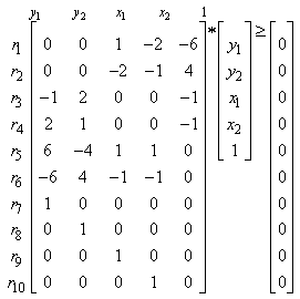 | (25) |
 | (26) |
 by rows
  and
and  , we have
 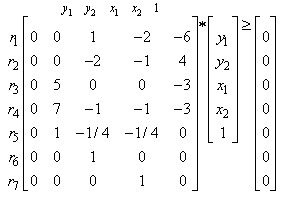 | (27) |
 are all positive, hence
  is only bounded below, the dual LP is unbounded above. For the primal LP, it is reduced to the following linear inequalities:
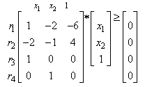 | (28) |
 and
and  , we can eliminate
  to obtain the both MLB and LUB for
  as
as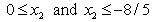 ; Consequently, the feasible interval for
  is
is , i.e., the primal LP has no solution !Example #5 LP with unbounded solutionConsider the LP:
 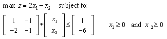 The corresponding HLFS for this LP as self-dual form [18] is:
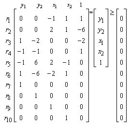 | (29) |
 and
and  , we can eliminate
  and obtain
 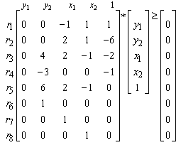 | (30) |
 , we have
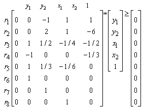 | (31) |
 and
and  , the 2nd column for
  and the last column for MLB and LUB,We obtain the feasible interval
  (i.e.,
  ) from rows
  and
and  as
as  and
and  Eliminate
  by rows
  and
and  and excluding the rows with dual variables
  and
and  only, we have inequalities for the primal variables
  and
and  as:
as: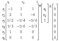 | (32) |
 , we have:
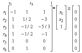 | (33) |
 from rows
  and
and  , we have
 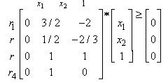 | (34) |
 , we have
 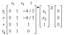 | (35) |
 is bounded below only with
  .Also
.Also  is not bounded above with LUB =
 . Hence, the feasible interval for
  is
is  .
. 5. GGE for Differential Varitional Inequalities (DVI)
- GGE may also be applied to linear space as a normed Banach space with an inner-product operator
 for solving variational inequalities (VI) or differential variational inequalities (DVI) as follows [15 and 16] or Variational-like Inequalities in Banach space [25 to 29]:Let
  where B is an
  matrix as a nonempty convex compact polyhedron in
  Let
Let  be a continuously differentiable function from
  into
into  with Jacobian
  .The variational inequality problem (VIP) associated with F and
  is to locate a solution
  in
in  satisfying the variational inequality (VI):
  in
in  . Note that in
  , we have
  Let the gap function associated with a VIP be defined for
  in
in  as:
as: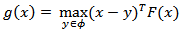 While the dual gap function associated with a VIP is defined as
 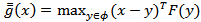 Using Newton’s first order Taylor linear approximation around a point
  in
in  , a linearized VIP as LVIP can be computed iteratively for
  as:
as: Consider the following nonconvex, nonlinear constrained mathematical program:
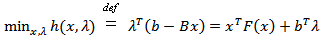 subject to
  Note that optimality occurs at:
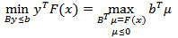 subject to:
 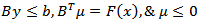 Consequently, we have the following homogeneous linear feasible system of inequalities
  Where
Where 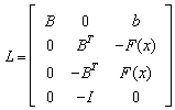 and
and  Note that
  can be resolved effectively for the feasible intervals of
  derived from
  as described and demonstrated by the proposed GGE algorithm illustrated in Section 3.
6. Conclusions and Future Work
- In conclusion, the author proposes a generalization of the traditional Gaussian elimination (GE) for solving system of linear equalities to compute the feasible intervals of all variables to resolve the feasibility of all linear systems with both equalities and/or inequalities included. This Generalized Gaussian Elimination (GGE) for linear systems is applicable to a wide range of engineering and scientific applications and is related closely to the NPC mystery of the operations research and solvability of differential variation inequalities (DVI). Furthermore, it can be shown that GGE is indeed a special case of GE and that both GGE and GE do share the same worst case computational complexity of
 where n is the number of variables and m is the number of constraints. This is accomplished by replacing the variable substitution of the Gaussian elimination method by variable transition such that a specific variable may be safely and recursively eliminated without losing its binding inequalities and preserving both the most lower bounds (MLB) and the least upper bound (LUB). It is shown that any system of linear system with mixed linear equalities and inequalities may be converted into its standard homogeneous form such that the proposed GGE algorithm may be applied to obtain the feasible interval of any variable of choice. From the feasible intervals of all the variables of a given linear system, one may determine whether or not it contains binary, integers, or mixed solutions. The correctness and validity of GGE is illustrated by solving sample linear programs with unique solution, unbounded solution, and no solution.Future work of this research includes the implementation of GGE as java code and Excel VB functions for very large system of linear inequalities or mixed of linear equalities and inequalities with millions of variables and/or constraints. The author is currently verifying a parameterized GGE algorithm for solving the linear Integer programming (LIP) problem as a potential alternative or replacement for the well known branch and bound (B&B) technique. A draft paper will be available for external review later. Funding from NSF or private foundations will be pursued to speed up the development of Java or VB functional codes for solving eigenvector systems, computing orthogonal basis, and DVI applications. GGE may also be applied to problems in operations research to reveal the availability of integer or binary solutions encountered in the NPC mystery as open issues.
ACKNOWLEDGEMENTS
- Generalization of the classical Gaussian elimination for linear systems to cover inequalities is the result of years of inquiry and discussion with Dr. Leone C. Monticone and Dr. William P. Niedringhaus, colleagues of the author at the MITRE Corporation where the author served as an aviation engineer. The author also was benefited professionally and intellectually from his colleagues, Dr. Leonard Wojcik and Mr. Matt McMahon during many years at the MITRE Corporation working on MITRE sponsored research (MSR) projects related to solving vary large linear systems. Review and editorial advice from SAP and AJCAM are also essential to the improved quality and readability of this paper.
 -Cocoercive Operators and Generalized Set-Valued Variational-Like Inclusions”, Journal of Mathematics, Vol. 2013, Article3 ID 738491, 10 pages.