Michael Gr. Voskoglou
School of Technological Applications, Graduate Technological Educational Institute (T. E. I.), Patras, Greece
Correspondence to: Michael Gr. Voskoglou, School of Technological Applications, Graduate Technological Educational Institute (T. E. I.), Patras, Greece.
| Email: |  |
Copyright © 2014 Scientific & Academic Publishing. All Rights Reserved.
Abstract
In the present paper we develop an improved version of the Triangular Fuzzy Model (TFM) for verifying the creditability of a chosen decision. The TFM is a variation of a special form of the Centre of Gravity (COG) defuzzification technique, which we have used in earlier papers as an assessment method in several human activities. The main idea of the TFM is the replacement of the rectangles appearing in the graph of the membership function of the COG method by isosceles triangles sharing common parts. In this way we cover the ambiguous cases of individuals’ scores being at the limits between two successive categories. A real application is also presented illustrating our results in practice, in which the outcomes of the TFM are compared with those of the COG technique and of other traditional methods (calculation of means and GPA index).
Keywords:
Decision making, Verification of a decision, GPA assessment index, Fuzzy logic, Center of gravity (COG) deffuzzification technique, Triangular Fuzzy Model (TFM)
Cite this paper: Michael Gr. Voskoglou, A Triangular Fuzzy Model for Decision Making, American Journal of Computational and Applied Mathematics , Vol. 4 No. 6, 2014, pp. 195-201. doi: 10.5923/j.ajcam.20140406.03.
1. Introduction
Decision Making (DM) is the process of choosing a solution between two or more alternatives, aiming to achieve the best possible results for a given problem. Obviously the above process has sense if, and only if, there exist more than one feasible solutions and a suitable criterion that helps the decision maker (d-m) to choose the best among these solutions. We recall that a solution is characterized as feasible, if it satisfies all the restrictions imposed onto the real system by the statement of the problem as well as all the natural restrictions imposed onto the problem by the real system; e.g. if x denotes the quantity of stock of a product, it must be x≥0. The choice of the suitable criterion, especially when the results of DM are affected by random events, depends upon the d-m‘s desired goals; e.g. optimistic or conservative criterion, etc.The rapid technological progress, the impressive development of the transport means, the globalization of the modern society, the enormous changes happened to the local and international economies and other similar reasons led during the last 50-60 years to a continuously increasing complexity of the our everyday life problems. As a result the DM process became in many cases a very difficult task, which is not possible to be based on the d-m’s experience, intuition and skills only, as it usually happened in the past. Thus, from the beginning of the 1950's a progressive development started of a systematic methodology for the DM process, which is based on Probability Theory, Statistics, Economics, Psychology, etc and it is known as Statistical Decision Theory.According to the nowadays existing standards the DM process involves the following steps:• d1: Analysis of the decision-problem, i.e. understanding, simplifying and reformulating the problem in a way permitting the application of the principles of DM on it.• d2: Collection from the real system and interpretation of all the necessary information related to the problem.• d3: Determination of all the alternative feasible solutions.• d4: Choice of the best solution in terms of the suitable (according to the d-m’s goals and targets) criterion.One could add one more step to the DM process, the verification (checking the creditability) of the chosen decision according to the results obtained by applying it in practice. However, this step is extended to areas, which due to their depth and importance for the administrative rationalism have become autonomous. Therefore, it is usually examined separately from the other steps of the DM process.Notice that the first three steps of the DM process presented above are continuous in the sense that the completion of each one of them usually needs some time, during which the d-m's reasoning is characterized by transitions between hierarchically neighbouring steps. The flow-diagram of the DM process is represented in Figure 1 below: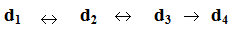 | Figure 1. The flow-diagram of the DM process |
Our target in the present paper is the development of an improved version of the Triangular Fuzzy Model (TFM) for verifying a taken decision. For this, the rest of the paper is organized as follows: In section 2 we present examples illustrating the process of DM under fuzzy conditions. In section 3 we apply, through a real example, two traditional methods for the verification of a taken decision (calculation of the means and GPA index), while in section 4 we use principles of Fuzzy Logic (FL) for presenting two alternative methods for the same purpose: A special form of the Center of Gravity (COG) defuzzification technique that has been used in earlier papers as a tool for assessing the individuals’ performance in several human activities and an improved version of the TFM, which is a variation of the COG method. The outcomes of the above - four in total - methods are compared to each other and explanations are given for the differences appeared among them. The last section 5 is devoted to our final conclusion and to a brief discussion about our future plans for further research on the subject.
2. DM under Fuzzy Conditions
In our everyday life a DM problem is frequently expressed in an ambiguous way involving a degree of uncertainty. In such cases the classical Statistical Decision Theory based on principles of the traditional bivalent logic (yes-no) is proved inadequate for helping the d-m for choosing the correct decision. On the contrary, FL, based on the notion of fuzzy sets introduced by Zadeh in 1965, offers a rich field of resources for this purpose by allowing the d-m to frame the goals and constraints of the decision problem in vague, linguistic terms, which may reflect the real situation. For general facts on FL we refer to the book [2]. The following examples illustrate the standard process of DM under fuzzy conditions:EXAMPLE 1: A company wants to employ as a sales manager the candidate with the best qualifications, provided that his/her request for salary is not very high and that his/her residence is in a close driving distance from the company’s place. They are four candidates for the above position, say Α, Β, C and D, with annual salary requests 29050, 25000, 14050, and 6250 euros respectively. Who of them is the best choice for the company under the above (fuzzy) conditions?In this DM problem we have the fuzzy goal (G) of employing the candidate with the best qualifications under the fuzzy constraints that his/her request for salary must not be very high (C1) and that his/her residence must be in a close driving distance from the companies place (C2). The steps of the DM process in such fuzzy situations are the following:Step 1: Choice of the universal set of the discourseIn our case we must obviously consider as universal set the set U = {A, B, C, D} of the four candidates.Step 2: Fuzzification of the decision problem’s dataIn this step the fuzzy goal and the fuzzy constraints of the problem are expressed as fuzzy sets in U. For this, we must define properly the corresponding for each case membership function. For example, the membership function  for the fuzzy constraint C1 can be defined by:
  =1 for s(x) < 6000,
  = 1 – 2 * 10 * s(x} for 6000 ≤ s(x) ≤ 30000 and
  = 0 for s(x) > 30000, where s(x) denotes the salary of the candidate x, for all x in U. Then
  (A) = 1 – 2 * 0.2905 = 0.419. Similarly we calculate the membership degrees of B, C and D and we write the constraint C1 as a fuzzy set in U in the form of the symbolic sum C1 = 0.419/A + 0.5/Β + 0.719/C + 0.875/D.In the same way (the relevant details are omitted here for reasons of brevity) we expressed the fuzzy goal G and the other fuzzy constraint C2 as fuzzy sets in U in the formG = 0.9/A + 0.6/B + 0.8/C + 0.6/D and C2 = 0.1/Α + 0.9/Β + 0.7/C + 1/D respectively1.Step 3: Evaluation of the fuzzy dataAccording to the Bellman-Zadeh’s criterion for DM in a fuzzy environment [1], the fuzzy decision F expressed as a fuzzy set in U is the intersection of the fuzzy sets G, C1 and C2 of U and the solution of the problem corresponds to the element x of U having the highest membership degree in F. In fact, it is logical to define a fuzzy decision as the choice that satisfies both the goals and the constraints and, if we interpret this as a logical “and”, we can model it with the intersection of all fuzzy goals and constraints of the decision problem. Finally we take the maximum of this set to obtain the best among the existing alternatives.But, it is well known that the membership function of the intersection
  is defined by
  for all x in U. Therefore it is easy to check that F = 0.1/A + 0.5/B + 0.7/C + 0.6/D.Step 4: Defuzzification The highest membership degree in F is 0.7 and corresponds to the candidate C. Therefore the candidate C is the best choice for the company. The fuzzy model of Bellman-Zadeh presented above can be further extended to accommodate the relative importance that could exist for the goal and constraints by using weighting coefficients. The following example illustrates this case:EXAMPLE 2: Reconsider Example 1 and assume that the Management Council of the company, taking into account the existing company’s budget, the results of the oral interviews of the four candidates and some other relevant factors, decided to attach weights 0.5, 0.2 and 0.3 to the goal G and to the constraints C1 and C2 respectively. Which will be the company’s decision under these conditions?In this case the membership function of the fuzzy decision F is defined through a linear combination of the weighted goal and constraints of the form
  , where mG (x),
  are the membership degrees in G, C1 and C2 respectively of each x in U (see Example 1) and the coefficients
  ,
,  and
and  are the weights attached to the fuzzy goal and constraints respectively, with
  =1 ([2], section 6.5). Therefore the membership degree of the candidate A in the fuzzy decision F in this case is mF (A) = 0.5 * 0.9 + 0.419 * 0.2 + 0.1 * 0.3 = 0.638. In the same way we find that mF (B) = 0.67, mF (C) = 0.7538 and mF (D) = 0.775. Therefore the candidate D will be the company’s choice in this case.
3. Traditional Methods for the Verification of a Chosen Decision
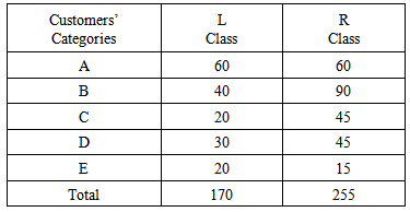
In this section we shall apply two traditional methods for verifying a chosen decision, the calculation of the means and the Grade Point Average (GPA) index. For this, let us consider the following real example:EXAMPLE: A car industry has decided to circulate its new model in the market in two different types, the luxury (L) Class and the regular (R) Class. Six months after the purchase of their cars the customers were asked to complete a written questionnaire concerning their degree of satisfaction for their new cars. Their answers were marked by the industry’s marketing department within a climax from 0 to 100 and they were divided in the following five categories according to the corresponding scores: A (90-100) = Full satisfied customers, B (75-89) = Very satisfied customers, C (60-74) = Satisfied customers, D (50-59) = Rather satisfied customers and E (0-49) = Unsatisfied customers. The scores assigned to the customers’ answers were the following:L Class: 100(5 times), 99(3), 98(10), 95(15), 94(12), 93(1), 92 (8), 90(6), 89(3), 88(7), 85(13), 82(4), 80(6), 79(1), 78(1), 76(2), 75(3), 74(3), 73(1), 72(5), 70(4), 68(2), 63(2), 60(3), 59(5), 58(1), 57(2), 56(3), 55(4), 54(2), 53(1), 52(2), 51(2), 50(8), 48(7), 45(8), 42(1), 40(3), 35(1).R Class: 100(7), 99(2), 98(3), 97(9), 95(18), 92(11), 91(4), 90(6), 88(12), 85(36), 82(8), 80(19), 78(9), 75(6), 70(17), 64(12), 60(16), 58(19), 56(3), 55(6), 50(17), 45(9), 40(6). The above data can be summarized as it is shown in Table 1:Table 1. Questionnaire’s data
 |
| |
|
The evaluation of the above data (verification of the industry’s decision about its new model) will be performed below using the above mentioned traditional methods.
3.1. Calculation of the Means
It is straightforward to calculate the means mL and mR of the scores of the customers’ answers for the Luxury and the Regular Class respectively, which are mL 76.006 and mR 75.09. This means that all the customers were very satisfied with their new cars, with the customers who purchased the L Class being better satisfied than those who purchased the R Class.
3.2. Application of the GPA Index
We recall that the GPA index is a weighted mean where more importance is given to the higher scores achieved, to which greater coefficients (weights) are attached. In other words the GPA index focuses on the quality “performance” rather, than on the mean “performance” of a group of individuals. For applying the GPA index on the data of our example let us denote by nA, nB, nC, nD and nE the number of the industry’s customers who belong to the above described categories A, B, C, D and E respectively and by n the total number of its customers. Then the GPA is calculated by the formula GPA = 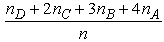 . Obviously we have that 0 ≤ GPA ≤ 4. In our case, using the data of Table 1 it is easy to check that both the GPA’s of the customers of the L Class and of the R Class are equal to
 2.529. Thus, according to the GPA index, the industry’s customers of the L Class and of the R Class were equally satisfied with their new cars.
4. Using Principles of FL for the Verification of a Chosen Decision
Here we refer again to the real example presented in the previous section. We shall use principles of FL to present the following two alternative methods for verifying the creditability of the chosen by the car industry decision:
4.1. The COG Method
This method is a special form of the commonly used in FL COG (or centroid) defuzzification technique. According to the COG technique the defuzzification of a fuzzy situation’s data is succeeded through the calculation of the coordinates of the COG of the level’s section contained between the graph of the membership function associated with this situation and the OX axis.In earlier papers ([3], [6], etc) the COG technique has been properly adapted for use as an assessment method of the individuals’ performance in several human activities. Here, using similar techniques, we shall adapt the COG technique for the verification of a chosen decision.For this, let us consider as universal set of our discourse the set U = {A, B, C, D, E} of the industry’s customers categories described in the previous section. We are going to represent the sets L and R of the customers who purchased the L Class and R Class respectively as fuzzy sets in U. For this, we define the membership function m: U → [0, 1] for both sets L and R in terms of the frequencies, i.e. by y = m(x) =  , where nx denotes the number of customers belonging to the category x in U and n denotes the total number of the customers of the corresponding set.Then, from Table 1 it turns out that L and R can be written as fuzzy sets in U in the form2:
 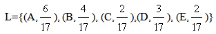 | (1) |
and 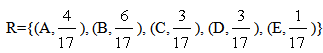 | (2) |
respectively.Now, we correspond to each xU an interval of values from a prefixed numerical distribution as follows: E → [0, 1), D → [1, 2), C → [2, 3), B → [3, 4), A → [4, 5]. This actually means that we replace U with a set of real intervals. Consequently, we have that y1 = m(x) = m(E) for all x in [0,1), y2 = m(x) = m(D} for all x in [1,2), y3 = m(x) = m(C) for all x in [2, 3), y4 = m(x) = m(B) for all x in [3, 4) and y5 = m(x) = m(A) for all x in [4,5). Since the membership values of the elements of U in L and R have been defined in terms of the corresponding frequencies, we obviously have that 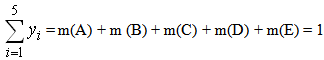 | (3) |
We are now in position to construct the graph of the membership function y = m(x), which has the form of the bar graph shown in Figure 2, wherefrom one can easily observe that the area of the level’s section, say F, contained between the bar graph of y = m(x) and the OX axis is equal to the sum of the areas of the five rectangles Fi , i =1, 2, 3, 4, 5. The one side of each one of these rectangles has length 1 unit and lies on the OX axis.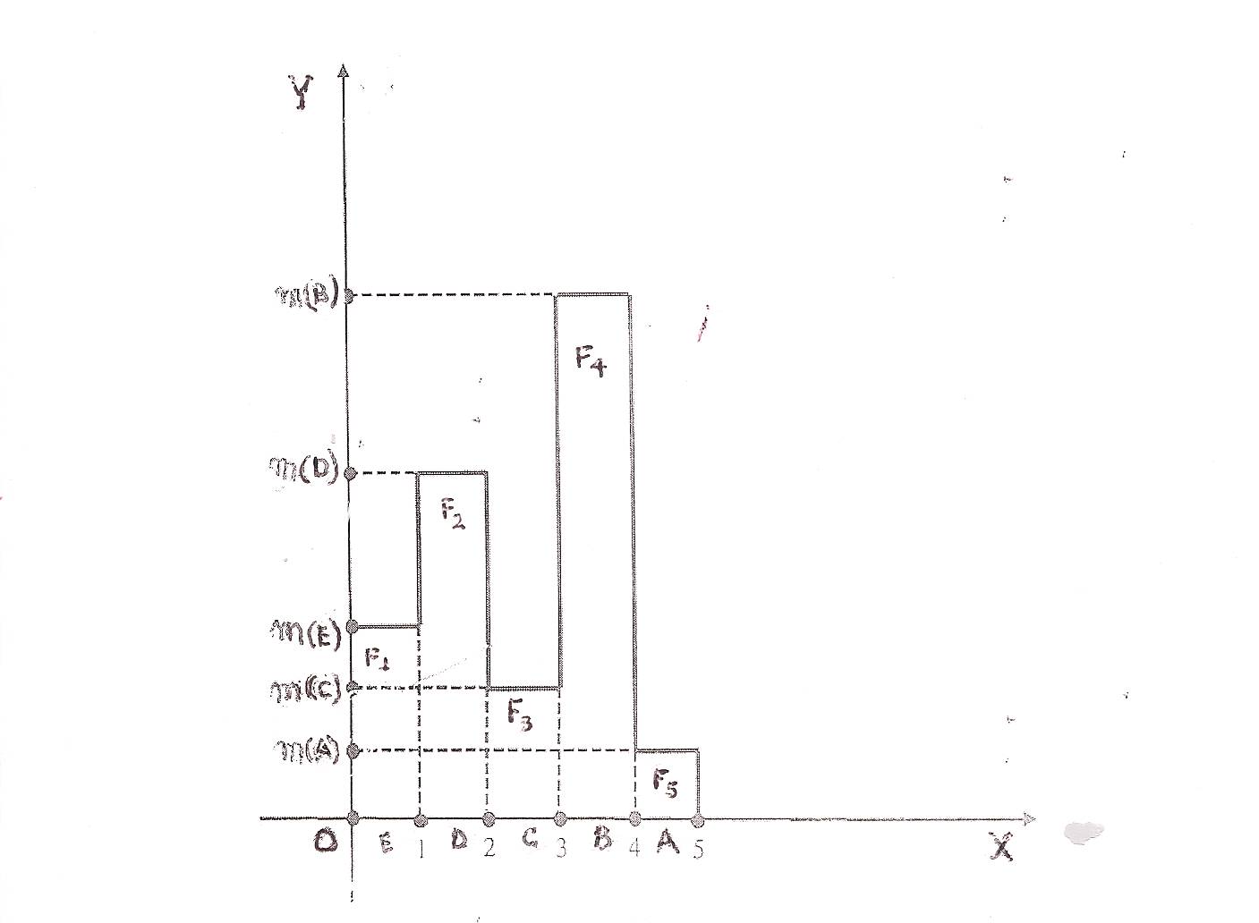 | Figure 2. Bar graphical data representation |
From Mechanics it is well known that the coordinates (xc, yc) of the COG, say Fc, of the level’s section F can be calculated by the formulas: 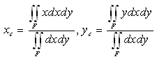 | (4) |
Taking into account the data represented by Figure 2 and equation (3) it is straightforward to check (e.g. see section 3 of [6]) that in this case formulas (4) can be transformed to the form: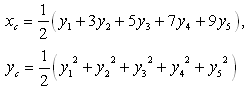 | (5) |
Then, using elementary algebraic inequalities it is easy to check that there is a unique minimum for yc corresponding to the COG Fm ( ) ([6], section 3). Further, the ideal case is when y1=y2=y3=y4=0 and y5=1. Then from the first of formulas (5) we find that xc =
  and yc =
  . Therefore the COG in this case is the point Fi(
 ,
, ). On the other hand the worst case is when y1=1 and y2=y3=y4= y5=0. Then from the first of formulas (5) we find that the COG in this case is the point Fw (
 ,
, ). Therefore the COG Fc of the level’s section F lies in the area of the triangle Fw Fm Fi .Then by elementary geometric observations ([9], section 3) one can obtain the following criterion: • Between the two groups of the industry’s customers the group with the biggest xc corresponds to the customers who are better satisfied with their new cars.• If the two groups have the same xc ≥ 2.5, then the group with the higher yc corresponds to the customers who are better satisfied with their new cars.• If the two groups have the same xc < 2.5, then the group with the lower yc corresponds to the customers who are better satisfied with their new cars.Substituting in formulas (5) the values of yi’s taken from forms (1) and (2) of the fuzzy sets L and R respectively it is straightforward to check that the coordinate xc of the COG for both L and R is equal to
  3.029 > 2.5. However, the coordinate yc is equal to
  for L and to
  for R. Therefore, according to the above stated criterion, the customers who purchased the R Class were better satisfied with their new cars than those who purchased the L class.
4.2. The Triangular Fuzzy Model (TFM)
The TFM is actually a variation of the above presented COG method. In the initial version of TFM developed in earlier papers [4-5] the individuals under assessment were divided in three assessment categories (A, B, C-E). In the improved version that we will develop here these categories are increased to five. In this way the model becomes more accurate.The main idea of TFM is the replacement of the rectangles appearing in the graph of the membership function of the COG method (Figure 2) by isosceles triangles sharing common parts (Figure 3). 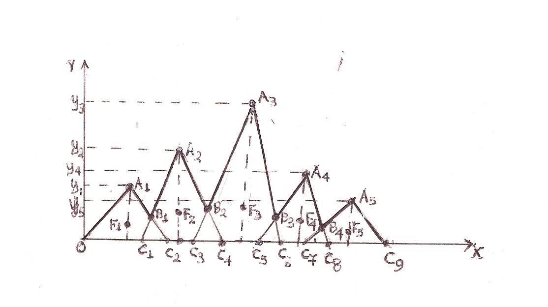 | Figure 3. The TFM’s scheme |
Therefore, in the TFM’s scheme (Figure 3) we have five such triangles, each one of them corresponding to a customer’s category (E, D, C, B and A respectively). Without loss of generality and for making our calculations easier we consider isosceles triangles with bases of length 10 units lying on the OX axis. The height to the base of each triangle is equal to the percentage of the industry’s customers who belong to the corresponding category. We allow for any two adjacent triangles to have 30% of their bases belonging to both of them. In this way we cover the ambiguous cases of the industry’s customers being at the limits between two successive categories (e.g. between A and B).The groups L and R of the customers who purchased the L Class and R Class respectively can be represented again, as we did in the COG method, as fuzzy set in U, whose membership function y=m(x) has as graph the line OA1B1A2B2A3 B3A4 B4A5C9 of Figure 3. It is easy to calculate the coordinates (bi1, bi2) of the points Bi, i = 1, 2, 3, 4, 5. In fact, B1 is the intersection of the straight line segments A1C2, C1A2, B2 is the intersection of C3A3, A2C4 and so on. Therefore, it is straightforward to determine the analytic form of y=m(x) consisting of 10 branches, corresponding to the equations of the straight lines OA1, A1B1, B1A2, A2B2, B2A3, A3B3, B3A4, A4B4, B4A5 and A5C9 in the intervals [0, 5), [5, b11), [b11, 12), [12, b21), [b21, 19), [19, b31), [b31, 26), [26. b41), [b41, 33) and [33, 38] respectively. However, in applying the TFM the use of the analytic form of y = m(x) is not needed (in contrast to the COG method) for the calculation of the COG of the resulting area. In fact, since the marginal cases of the customers’ categories should be considered as common parts for any pair of the adjacent triangles, it is logical to not subtract the areas of the intersections from the area of the corresponding level’s section, although in this way we count them twice; e.g. placing the ambiguous cases B+ and A- in both regions B and A. In other words, the COG method, which calculates the coordinates of the COG of the area between the graph of the membership function and the OX axis (see Figure 3), thus considering the areas of the “common” triangles C1B1C2, C3B2C4, C5B3C6 and C7B4C8 only once, is not the proper one to be applied in the above situation. Indeed, in this case it is reasonable to represent each one of the five triangles OA1C2, C1A2C4, C3A3C6, C5A4C8 and C7A5C9 of Figure 3 by their COG’s Fi, i=1, 2, 3, 4, 5 and to consider the entire area defined in this way as the system of these points-centers. More explicitly, the steps of the whole construction of the TFM are the following:1. Let yi, i=1,2,3,4,5 be the percentages of the industry’s customers belonging to the categories E, D, C, B, and A respectively; then  =1 (100%).2. We consider the isosceles triangles with bases having lengths of 10 units each and their heights being equal to yi,, i=1,2,3,4,5 in the way that has been illustrated in Figure 3. Each pair of adjacent triangles has common parts in the base with length 3 units.3. We calculate the coordinates
  of the COG Fi, i=1,2,3, 4, 5 of each triangle as follows: The COG of a triangle is the point of intersection of its medians, and since this point divides the median in proportion 2:1 from the vertex, we find, taking also into account that the triangles are isosceles, that
  . Also, since the triangles’ bases have a length of 10 units, we observe that xci=7i-2.4. We consider the system of the centers Fi, i=1, 2, 3 and we calculate the coordinates (Xc, Yc) of the COG F of the whole area S considered in Figure 3 by the following formulas, derived from the commonly used in such cases definition:
 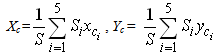 | (6) |
In formulas (6) Si, i= 1, 2, 3, 4, 5 denote the areas of the corresponding triangles. Therefore Si = 5yi and 
 . Thus, from formulas (6) we finally get that
 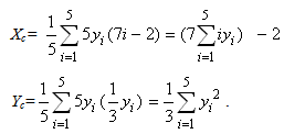 | (7) |
5. We determine the area where the COG F lies as follows : For i, j=1, 2, 3, 4, 5, we have that 0 ≤ (yi –yj)2=yi2+yj2-2yiyj, therefore yi2+yj2  2yiyj, with the equality holding if, and only if, yi=yj. Therefore
 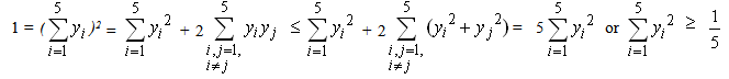 | (8) |
with the equality holding if, and only if, y1 = y2 = y3 = y4 = y5 =  . In the case of equality the first of formulas (7) gives that
  . Further, combining the inequality (8) with the second of formulas (7) one finds that
  Therefore the unique minimum for Yc corresponds to the COG Fm (15,
  ).The ideal case is when y1=y2=y3= y4=0 and y5=1. Then from formulas (7) we get that Xc = 33 and Yc =
  . Therefore the COG in this case is the point Fi (33,
  ). On the other hand, the worst case is when y1=1 and y2= y3 = y4= y5=0. Then from formulas (2), we find that the COG is the point Fw(5,
  ). Therefore the area where the centre of gravity Fc lies is the area of the triangle Fw Fm Fi . (Figure 4)6. We formulate our assessment criterion as follows: From elementary geometric observations (Figure 4) it follows that for the two groups of the industry’s customers the group having the greater Xc corresponds to the customers who are better satisfied with their new cars. Further, if the two groups have the same Xc ≥15, then the group having the COG which is situated closer to Fi is the group with the higher Yc. Also, if the two groups have the same Xc<15, then the group having the COG which is situated farther to Fw is the group with the lower Yc.
  | Figure 4. The area where the COG lies |
Based on the above considerations it is logical to formulate our criterion for comparing the two groups in the following form: • Between the two groups of the industry’s customers the group with the biggest Xc corresponds to the customers who are better satisfied with their new cars.• If the two groups have the same Xc ≥ 15, then the group with the higher Yc corresponds to the customers who are better satisfied with their new cars.• If the two groups have the same Xc < 15, then the group with the lower Yc corresponds to the customers who are better satisfied with their new cars.Substituting in formulas (7) the values of yi’s taken from the forms (1) and (2) of the fuzzy sets L and R respectively (section 4.1) it is straightforward to check that the coordinate Xc of the COG for both L and R is equal to  23.294>15. However, the coordinate Yc is equal to
  for L and to
  for R. Therefore, according to the above stated criterion, the customers who purchased the R Class were better satisfied with their new cars than those who purchased the L Class.
4.3. Comparison of the Methods Applied
In sections 3 and 4 we applied four different methods for verifying the creditability of the car industry’s decision about its new model. According to the outcomes of all these methods, the above decision was proved to be satisfactory. In fact, the means in the first method were greater than 75 (very satisfied customers), while the value 2.529 of the GPA index in the second method is close enough to its maximum possible value 4. Also the values of the abscissa of the COG method and the TFR (3.029 and 23.294 respectively) are close enough to the corresponding values of the ideal case (4.5 and 33 respectively).However, differences appeared among the outcomes of the above methods concerning the degree of satisfaction of the customers who purchased the L Class and the R Class respectively. In fact, the calculation of the means demonstrated a slightly higher degree of satisfaction for the customers of the L Class, while according to the GPA index the customers were equally satisfied in both cases. On the contrary, the two FL methods (COG and TFM) demonstrated a slightly higher degree of satisfaction for the customers of the R ClassThe above differences are not embarrassing, because, in contrast to the calculation of the means which focuses on the mean behaviour (performance) of the two groups of customers, the other three methods (GPA, COG and TFM) focus on their quality behaviour by assigning greater weight coefficients to the higher scores achieved by the customers.In fact, the formula calculating the GPA index (section 3.2) can be written in our case in the form | (9) |
Further, since in COG and TFM the behaviour of a group is assessed by the value of the abscissa of the corresponding COG, observing the first of formulas (5) and (7) and formula (9) we can form the following Table:Table 2. Weight coefficients of the yi’s
 |
| |
|
From Table 2 becomes evident that TFM assigns greater coefficients to the higher with respect to the lower scores than COG and also COG does the same thing with respect to GPA. In other words TFM is more sensitive than COG, and COG is more sensitive than GPA for assessing the quality behaviour of a group.In concluding, it is suggested to the user to choose among the above methods the one that fits better to its personal criteria of goals.
5. Discussion
The first two of the metods applied above for verifying the creditability of a chosen decision (calculation of the means and GPA index) are based on principles of the classical (bivalent) logic, while the other two methods (COG and TFM) are based on principles of FL. The TFM is a recently developed variation of the COG method. Consequently, there is a need to be applied in more real examples of decision problems in future for obtaining safer conclusions about its advantages/disadvantages with respect to the COG method. This is among the priorities of our future research plans. On the other hand, since the TFM approach appears to have the potential of a general assessment method, our future research plans include also the effort of applying this approach in assessing the individuals’ performance in various other human activities.
6. Conclusions
Two are the innovations of this paper: First we developed an improved version of the TFM for verifying the creditability of a chosen decision .and second it was shown that TFM is more sensitive to the higher scores than the other assessment methods used.
Notes
1. We recall that the definition of the membership function is usually depending on empirical or statistical data collected from a sample of the population that we study. However a necessary condition for the creditability of the fuzzy model in representing the corresponding real situation is that the choice of the membership function is compatible with the common logic.2. We recall that a fuzzy set can be symbolically written in several forms, e.g. as a symbolic sum (see section 2), as a set of ordered pairs (see above), etc.
References
| [1] | Bellman, R. E. & Zadeh, L. A., “Decision making in fuzzy environment”, Management Science, 17, 141-164, 1970. |
| [2] | Klir, G. J. & Folger, T. A., “Fuzzy Sets, Uncertainty and Information”, Prentice-Hall, London, 1988. |
| [3] | Subbotin, I. Ya., Badkoobehi, H., Bilotckii, N. N., “Application of fuzzy logic to learning assessment”, Didactics of Mathematics: Problems and Investigations, 22, 38-41, 2004. |
| [4] | Subbotin, I. Ya., Bilotskii, N. N., “Triangular fuzzy logic model for learning assessment”, Didactics of Mathematics: Problems and Investigations, 41, 84-88, 2014. |
| [5] | Subbotin, I. Ya, Voskoglou, M. Gr., “A Triangular Fuzzy Model for Assessing Students’ Critical Thinking Skills”, International Journal of Applications of Fuzzy Sets and Artificial Intelligence, 4, 173-186, 2014. |
| [6] | Voskoglou, M. Gr., “A Study on Fuzzy Systems”, American Journal of Computational and Applied Mathematics, 2(5), 232-240, 2012. |
 Abstract
 Reference
 Full-Text PDF
 Full-text HTML