1. Introduction

Fourier series is one of the most important tools in applied sciences. For example one can solve partial differential equations using Fourier series. Further one can find the sum of certain numerical series using Fourier series. Fractional partial differential equations appeared to have many applications in physics and engineering. There are many definitions of fractional derivative. One of the most recent ones is the conformal fractional derivative [5].

Recently [1], fractional Taylor power series was introduced, and a beautiful theory was layed there. However, no work is done on fractional Fourier series, though there is some work on fractional fourier transform.

The aim of this paper is to introduce conformable fractional Fourier series. As an application we solve some fractional partial differential equations using fractional Fourier series.

For more applications on conformable fractional derivative we refer to [2-4].

2. Basics of Conformable Fractional Derivative

The subject of fractional derivative is as old as calculus. In 1695, L’Hopital asked if the expression has any meaning. Since then, many researchers have been trying to generalize the concept of the usual derivative to fractional derivatives. These days, many definitions for the fractional derivative are available. Most of these definitions use an integral form. The most popular definitions are:

(i) Riemann - Liouville Definition: If is a positive integer and , the αth derivative of f is given by

(ii) Caputo Definition. For , the α derivative of is

Now, all definitions are attempted to satisfy the usual properties of the standard derivative. The only property inherited by all definitions of fractional derivative is the linearity property. However, the following are the set- backs of one definition or another:

(i) The Riemann-Liouville derivative does not satisfy for the Caputo derivative), if α is not a natural number.

(ii) All fractional derivatives do not satisfy the known product rule:

(iii) All fractional derivatives do not satisfy the known quotient rule:

(iv) All fractional derivatives do not satisfy the chain rule:

(v) All fractional derivatives do not satisfy: in general

(vi) Caputo definition assumes that the function is differentiable.

(vii) , for all constant functions .

In a new definition called conformable fractional derivative was introduced.

Definition. If α > 0 then we define

where is the ceiling of α. We call the fractional derivative of of order α. We shall write for .

The new definition satisfies:

1. , for all

2. , for all constant functions .

Further, for and be α-differentiable at a point , with Then

3.

4.

We list here the fractional derivatives of certain functions, for the purpose of comparing the results of the new definition with the usual definition of the derivative:

1. 2.1.

2.2.

2.3.

2.4.

On letting in these derivatives, we get the corresponding ordinary derivatives.

One should notice that a function could be α-differentiable at a point but not differentiable, for example, take. Then . Hence . But does not exist. This is not the case for the known classical fractional derivatives.

3. Fractional Fourier Series

Let and be defined by

and be any function. Let be defined by

For example, if , then

Definition 3.1. A function is called α-periodical with period if

for all

As an example, is α-periodic with period

Definition 3.2. Two functions are called α-orthogonal on if

Examples 3.1. and are α-orthogonal on .

Proof. Put . Then

Further, when t = 0, x = 0, and when , x = 2π. Hence

In general, using the idea in example 3.1 one can easily prove:

Theorem 3.1.

(i) and are orthogonal on , for all n ≠ m.

(ii) and are orthogonal on , for all n ≠ m.

(iii) and are orthogonal on , for all n, m.

Now let us define the Fourier coefficients of an α-periodic function with period p.

Definition 3.3. Let f: be a given peicewise continuous α-periodic with period p: Then we define:

(i) The cosine α-Fourier coefficients of f as

(ii) The sine α-Fourier coefficients of f as

For example, the cosine -Fourier coefficients of the function is: a₁ = 1, and a_n = 0 for all n ≠ 1, where , .

Now, we give the definition of the fractional Fourier series:

Definition 3.4. Let f: be a given peicewise continuous function which is α-periodical with period p: Then the α-fractional Fourier series of f associated with the interval [0, p] is

where a_n and b_n are as in Definition 3.3

Let us have some examples.

Example 3.2. Let , and ,

with p = π² on the interval [0, π²]: Then,

Using change of variables: , we get , θ = 0 if t = 0, t = 0, θ = π

if , and θ = 2π if t = (π)². Hence, the integral becomes

Similarly

So,

Example 3.3. Let

Then

and

Hence

One can easily prove the following classical result.

Theorem 3.2. The fractional Fourier series of a piece wise continuous α- periodical function converges pointwise to the average limit of the function at each point of discontinuity, and to the function at each point of continuity.

4. Applications

In this section we will use fractional Fourier series to solve some fractional partial differential equations. Namely, we will solve the equation

(4.1)

(4.2)

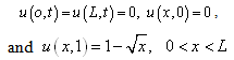(4.3)

Solution. We will use separation of variables technique.

So let . Substitute in the equation to get

From which we get

Since x and t are independent variables, then we get , constant to be determined. Hence

(4.4)

and

(4.5)

Conditions (4.3) suggests that we work with equation (4.4) first.

There are three possibilities for λ:

(i) λ = 0. Then equation (4.4) becomes , and from the property (2) of conformable fractional derivative, we get . Condition (4.3) shows that c = 0:

(ii) λ > 0. Then equation (4.4) becomes , and from formula (2.4) of the conformable fractional derivative, we get 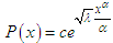. Condition (4.3) shows that c = 0:

(iii) λ < 0. Then equation (4.4) becomes . Using formulas (2.2) and (2.3) we get

(4.6)

Condition (4.3) implies that c₁ = 0. So . Another use of condition (4.3) gives . Hence

(4.7)

So

(4.8)

Now, we go back to equation (4.5) to get . Using formula (2.4) we get

(4.9)

Condition (4.3) implies that a₂ = - a₁. Hence

(4.10)

Combining (4.8) and (4.10) to get

(4.11)

Now, using the condition , to get

Using the α - Fourier series of 1 - xα, we find b_n