H. I. Okagbue, S. O. Edeki, A. A. Opanuga
Department of Mathematics, College of Science & Technology, Covenant University, Otta, Nigeria
Correspondence to: S. O. Edeki, Department of Mathematics, College of Science & Technology, Covenant University, Otta, Nigeria.
| Email: |  |
Copyright © 2014 Scientific & Academic Publishing. All Rights Reserved.
Abstract
This work provides a simulation-based approach of assessing the risk and uncertainty involved in estimating the expected earnings of an organization. The procedure involves using Monte Carlo Simulation (MCS) in creating various possible outcomes and scenarios. The MCS is found to be more effective than single point estimates or guesswork. Hence, it is an efficient and useful tool in risk management analysis. The analysis of the output of the simulation reveals that the expected earnings is a little bit lower than the most likely forecasted value of N30m but there is 37% chance that the expected earnings might drop below or rise above the estimated value by margin of N10.9m and the wide range of possible outcomes make the venture to be very risky as uncertainties in unit sales, unit price or variable cost can push the earnings to assume any value within the wide range. It is also observed that a large increase in the unit sales and a moderate increase in the unit price will increase the expected revenue which will in turn increase the earnings. The regression analysis gives almost the same result as MCS.
Keywords:
Monte Carlo Simulation, Risk Analysis, Expected Earnings
Cite this paper: H. I. Okagbue, S. O. Edeki, A. A. Opanuga, A Monte Carlo Simulation Approach in Assessing Risk and Uncertainty Involved in Estimating the Expected Earnings of an Organization: A Case Study in Nigeria, American Journal of Computational and Applied Mathematics , Vol. 4 No. 5, 2014, pp. 161-166. doi: 10.5923/j.ajcam.20140405.02.
1. Introduction
Business environment involves risk, and we often have difficulty in estimating the expected earnings of an organization, especially for the upcoming year. In finance, there is a fair amount of uncertainty and risk involved when estimating the future values of figures (expected earnings and revenues) due to wide variety of potential outcomes. Most organizations give a single point estimate of their projected earnings which may be misleading [1]. Some even resort to guesswork or trial and error method. This is also is a poor method. We live in an environment faced with risk and operate our businesses in a risky world, as higher rewards only come with risks. Planning in any organization is risky when the elements of risk are neglected. The availability of computers has made simulation possible; some of these techniques include Monte Carlo Simulation used in this paper. It helps in creating and forecasting the future (expected earnings) while investigating the risk involved in the process. MCS is a technique that converts uncertainties in input variables of model into probability distributions. It is a very effective technique, widely accepted for true results [2]. It is characterized by a unique feature for running multiple simulations by using multiple randomly generated numbers for the prediction of outcomes for risk variables [3]. It is used as a substitute for numerical integration [4-5]. The MCS as a class of computational algorithms depend on a repeated random sampling to obtain numerical results.Jonathan in [6] wrote that risk and uncertainty are very different animals, but they are of the same species, the lines of demarcation are often blurred. Risk is something one bears and it is the outcome of uncertainty. Only using the results from an uncertainty simulation analysis like Monte Carlo Simulation and finding ways to hedge or mitigate the quantified fluctuations and downside risk of the organization’s market performance in this work, would be constructed as having performed risk analysis and management.Risk can be seen as any uncertainty that affects a system in an unknown fashion whereby the ramifications are also unknown but bears with it great fluctuation in value and outcome [6-7]. What we can do to understand risks better is through a systematic assessment of measuring, monitoring and managing risks, otherwise simply noting that risks exist and moving on is not optional [8]. Risk analysis is a technique for enhancement of results and not an alternative for standard investment appraisal methodology [3]. Edeki et al noted the effects of stochastic capital reserve on actuarial risk analysis with regard to ruin and survival probabilities [9].Knight in [3] argued that risk and certainty were initially not the same; stressing that risks cover events whose outcomes are known or can be quantified as a result of historical evidence and probability distribution. Many researchers reject the validity of Knight’s view to risks [10-12].
2. Formulation of the Mathematical Problem & Model Description
In this section, we describe the problem to be solved, objectives of the study and a brief but concise description of the model to be used.The research work is based on the application of MCS to a probabilistic model which bears a risk.
2.1. Formulation of the Mathematical Problem
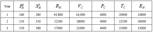
A big sized bakery located at Ogudu G.R.A., Lagos, Nigeria, owned by a promising entrepreneur was faced with the problem of assessing the risk involved in calculating the expected earnings in the coming year. He wanted to know exactly how their market performance will be before he can talk of diversification, expansion, recruitment of staff etc. He was very concerned with the uncertainties in the prices of the raw materials like wheat flour, butter, sugar, yeasts, vegetable oil, others and the diesel used in powering the bakery in the absence of power.Based on their market performance for the past 3 years, the manager then assumed that their revenue and earnings before tax will be the data shown below:We denote Unit price as  , Unit sales as
  , Revenue as
  , Variable cost as
  , Fixed cost as
  , Total costs as
  , Earnings as
  , and Costs
  , (all in
  ’000:00).
Table 1. Market performance for the last 3 years
 |
| |
|
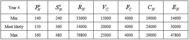
Table 2. Forecasted Market Performance
 |
| |
|
We define the Earnings before income tax as: | (1) |
2.2. Objectives of the Research
a. We will be investigating how the uncertainty in the unit price, unit sales and variable costs affect the expected earnings.b. Comparing the single point estimate and the Monte Carlo various possible outcomes and scenarios and then drawing conclusion.c. Investigating the amount of risk involved in predicting the earning of the organization.d. Demonstrating the use of Monte Carlo Simulation as an efficient risk management tool and evaluating its forecasting power.e. Calculate the amount of risks using different methods like; probability of occurrence, standard deviation, volatility etc.f. Critical examination of the behavior of our distribution at small samples, which is area of interest because theoretical substantiation for most parametric inference techniques is based on large sample theory [13-15].g. Making inference on the comparison of the theoretical and the simulated results of all the variables of the model.h. Running a convergence test to determine the efficiency of the Monte Carlo method and also comparing it and regression forecasts.
2.3. Model Description and Methodology


 Thus, for a fixed cost of
  4000, (1) becomes:
 | (2) |
The variables in the model based on the above table follow a triangular distribution. The triangular distribution describes a situation where the minimum, maximum and most likely value are known to occur. The most likely value falls between the minimum and maximum value forming a triangular – shaped distribution, which shows that values near the minimum and maximum are likely to occur than those near the most likely value.The research was carried out by simulation. The aim being to recreate many artificial scenarios based on the collected data. The data was collected from a bakery. The mode of data collection was manual.Since a model has been assumed and the variables are identified to follow triangular distribution which is just an improvement on the uniform distribution, we are going to simulate the variables using the SPSS 17.0. It is important to note that since we do not have data points on the SPSS data window, we must write a program for the simulation. Henceforth, a program was written and run on the syntax window to generate the required data. In this case, we simulate for the unit price (140,160), the unit sales (240000, 480000), and the total cost (15000000, 25000000).The variables are arranged in columns with their corresponding data points in rows on a spreadsheet form. The outputs show that the computer randomly resamples the data and the descriptive as it would be seen later are closer to the forecasted values based on the model.
3. Data Analysis: The Simulated and the Theoretical Results
3.1. Comparison between the Simulated & Theoretical Results at both Large & Small Samples
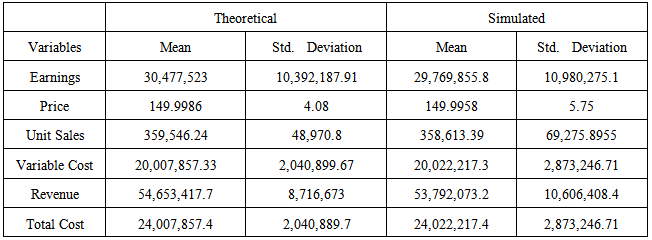
Before any analysis is done, we first of all compare the results of the simulated data with that of the theoretical data. This is done by substituting the values obtained from the simulation into the equations of the triangular distribution to determine the mean and the standard deviation respectively, since the model assumptions is based on the fact that all the variables follow the triangular distribution. The aim of this comparison is to investigate whether the simulated values of all the variables are close to their corresponding theoretical values. The theoretical results was based on the following formulae of the triangular distribution  | (3) |
 | (4) |
where  is simulated minimum,
  is simulated mean, and
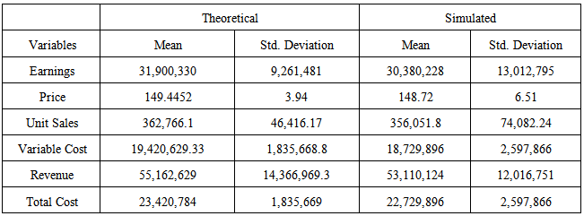
  is simulated maximum.It can be clearly seen that the values of both the simulated and the theoretical are closer on their average values than their standard deviation when compared together.Apart from the high standard deviations of the respective variables, the theoretical values differs greatly from the simulated one, meaning that the smaller the sample size, the higher the bias. This implies that the higher the sample size, the more efficient Monte Carlo Simulation becomes in estimating the various variables.
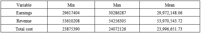
 Table 3. Comparison between the Theoretical & Simulated results at large sample
 |
| |
|
Table 4. Comparison between the theoretical & simulated results at small sample
 |
| |
|
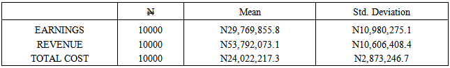
Table 5. Descriptive for the Earnings
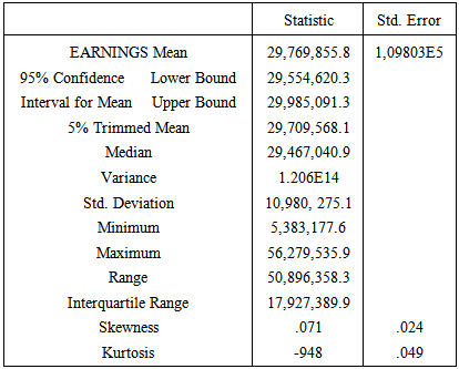 |
| |
|
Measurement of RiskStandard deviation of the earnings is  10,980,275Coefficient of Variation: Coefficient of Variation (CV) is simply the ratio of Standard Deviation to the mean i.e. the measure of risk per unit earnings, or when inverted can be used as a measure of earnings per unit of risk. Thus, for profit optimization, we will be interested in minimizing the CV and maximizing the inverse of the CV:
 and
and 
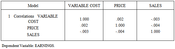
Table 6. Coefficient Correlations of the Independent Variables
 |
| |
|
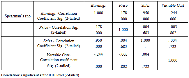
Table 7. Nonparametric Correlations
 |
| |
|
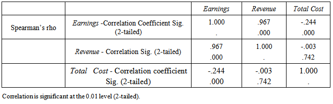
Table 8. Nonparametric Correlations
 |
| |
|
Table 9. Summary of analysis of the Kolmogonov – Simorov test for the 2 distribution
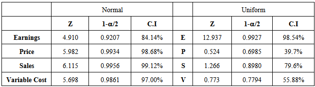 |
| |
|
Table 10. Model Summary for the Regressionb
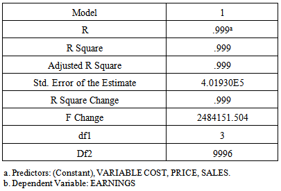 |
| |
|
Table 11. Comparison of the forecasted earnings of MCS and Regression
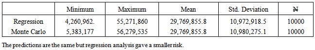 |
| |
|
Table 12. Summary of the effects of P.S.V. on E
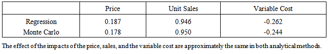 |
| |
|
Table 13. MCS Convergence test
 |
| |
|
Table 14. The analyses are summarized as follows
 |
| |
|
3.2. Discussion of Results
Here, we will briefly discuss and highlight the key findings as revealed by the analysis of our results as follows:a. Values of both the simulated and the theoretical are closer on their average values than their standard deviation when compared together at large samples.b. Apart from the high standard deviations of the respective variables, the theoretical values differs greatly from the simulated one, meaning that the smaller the sample size, the higher the bias. This implies that the higher the sample size, the more efficient Monte Carlo Simulation becomes in estimating the various variables.c. The expected earnings are likely to be N29,769,855. We are also 95% confident that the expected earnings, the standard deviation is estimated to be N10,980,275 which is the measure of risk. The large SD implies that there is high probability that the expected earnings might drop below or rise above the forecasted earnings which is very risky especially when it falls below the forecasted earnings. Also the wide range of N50, 896,358 means that the expected earnings can assume a wide range of values which can be lower or higher. Also this is very risky as uncertainties in unit price, unit sales or variable costs can push the earnings to assume any value within the wide range.d. The minimum and maximum values of the simulated earnings are in variance with their respective forecasted values.e. The skewness equals 0.071 means there is a small probability of expecting lower earnings.f. The Kurtosis estimate is – 0.948 which means that we will expect large losses/gains-that is, the probability of having the outliers as our potential earnings despite the uncertainties in the unit price, unit sales or variable costs, this is as a result of the thinner shape of the distribution and few outliers. Statistically, it implies that the probability of the earnings to assume values outside the range is small.g. The coefficient of variation CV equals 0.37 means that there is 37% chance that the expected earnings can deviate by N10,980,275.h. The correlation between the unit sales & earnings and between unit price & expected earnings is positive. Variable costs and earnings, on the other hand, are negatively correlated.i. The correction between the revenue and the expected earnings is positive. Total cost and earnings, on the other hand, are negatively correlated.j. The price and the variable cost are positively correlated. While the unit sales and the variable cost are negatively correlated. Also the price and the unit sales are negatively correlatedk. Kolmogorov-Smirnov test reveals that all the simulated data approximately fits the normal distribution.l. Comparison between MCS and regression reveals that the model actually fits; the forecast are almost the same but regression analysis gives a higher risk. The effects of the impacts of the price, sales, and the variable cost on the earnings are approximately the same in both MCS and Regression.m. The result of the convergence test shows that the simulation falls between the accepted ranges and hence, the simulated data are closer to the forecast one.
4. Conclusions and Recommendations
From the analysis, Monte Carlo Simulation is straight forward and flexible in application. However, it cannot wipe out uncertainty and risk, but it makes them easier to be understood by ascribing probabilistic characteristics to the inputs and the outputs of a model. It can be very helpful for determining different risks and factor that affect forecasted variables and, therefore, leads to accurate predictions. As seen, it was used to recreate and recover a process, thereby creating a scenario comparable with the forecasted data. MCS estimate as compared to a single value estimate is more accurate and effective. The uncertainties in the unit price, the unit sales, and the variable costs affect the expected earnings positively or negatively. MCS also provides a probability of the entire earnings outcomes allowing the decision makers to explore any pertinent scenarios associated with their expectation. Finally, MCS provides managers with critical information on which risk factors and assumptions that are driving the projected probability of earnings outcomes, giving them all important feedback they need to focus their resources on, addressing those risk assumptions that will have the greatest positive impact on their business, improving their efficiency and profit optimization.The firm is therefore, advised to plan effectively since there are chances that the expected earnings might fall or rise above the forecasted. Hence, to ensure profitability, they should improve on the quality to maximize unit sales at a more customer friendly price. On the other hand, they should devise ways to minimize production costs, since the estimated value are unlikely to deviate greatly as seen in the analysis.
ACKNOWLEDGEMENTS
The authors are grateful to the anonymous reviewers and referees for their valuable comments and helpful suggestions towards the improvement of the paper.
References
| [1] | T. Lordanova, Managing uncertainties in Business. Wiley & Sons. New York, 2004. |
| [2] | Z. M. Christopher, ‘‘Monte Carlo Simulation, Quantitative Applications in the Social Sciences’’, Sage University Paper Series, 116, 1997. |
| [3] | F. H. Knight, ‘‘Risk, Uncertainty and Profit’’, Houston Mifflin, Boston, 1921. |
| [4] | P. P. Boyle, ‘‘Options: a Monte Carlo Approach’’, Journal of Finantial Economics 4, (1977), 323-338. |
| [5] | P. Boyle, M. Broadie and P. Glasserman, ‘‘Monte Carlo Methods for Security Pricing’’, Journal of Economics Dynamics and Control, vol (8-9), (1997), 1267-1231. |
| [6] | M. Jonathan., Real Option Analysis Course: Business Cases. Wiley & Sons, New York, (2003). |
| [7] | M. Jonathan, Modeling Risk. Wiley & Sons. New York, (2006). |
| [8] | B. Dupire, Pricing and Risk Management. Risk Books, (1998). |
| [9] | S. O. Edeki, I. Adinya, O. O. Ugbebor, ‘‘The Effect of Stochastic Capital Reserve on Actuarial Risk Analysis via an Integro-differential Equation’’, IAENG International Journal of Applied Mathematics 44 (2), (2014): 83-90. |
| [10] | K. Bock, and S. Truck ‘’Assessing Uncertainty and Risk in Public Sector Investment Projects’’, Technology and Investment, 2011 (2), 105-123. (www.SciRP.org/journal/ti) |
| [11] | S. F. le Roy and D. Singell, ‘‘Knight on Risk and Uncertainty’’, The Journal of Political Economy, 95, (2), 1987, 394-406. doi:10.1086/261461 |
| [12] | M. Friedman, ‘‘Price Theory: A Provisional Text’’, Aldine, Chicago, 1976. |
| [13] | G. Cicchitelli, ‘‘On the Robustness of one-sample t-test’’. Journal of Statistical Computation and Simulation, (1989) |
| [14] | B. S. Everitt, ‘‘A Monte Carlo Investigation of the robustness of Hotelling’s one –and two-sample T2 tests’’, Journal of the American Statistical Association, (1979). |
| [15] | D. F. Hendry and R.W. Harrison, ‘‘Monte Carlo Methodology and the finite sample behavior of ordinary and two-stage least squares’’, Journal of Econometrics, (1974). |
 Abstract
 Reference
 Full-Text PDF
 Full-text HTML