M. Y. Adamu, E. Suleiman
Mathematical Sciences Programme, Abubakar Tafawa Balewa, University, Bauchi, Nigeria
Correspondence to: M. Y. Adamu, Mathematical Sciences Programme, Abubakar Tafawa Balewa, University, Bauchi, Nigeria.
| Email: |  |
Copyright © 2014 Scientific & Academic Publishing. All Rights Reserved.
Abstract
A class of bilinear differential operators is discussed. Some bilinear differential equations which generalized Hirota bilinear equations are used through assigning appropriate signs. We formulate a more general bilinear equation with mix DƤ –operators using different natural numbers P = 5. The resulting bilinear differential equations are identified by a special kind of Bell polynomials, and also the linear superposition principle is applied to the construction of their linear subspaces of solution. We have also given amore examples by algorithm using weights of dependent variable.
Keywords:
Bilinear Equations, Bell Polynomial, Superposition Principle, N-wave Solutions
Cite this paper: M. Y. Adamu, E. Suleiman, On Bilinear Equations, Bell Polynomials and Linear Superposition Principle, American Journal of Computational and Applied Mathematics , Vol. 4 No. 5, 2014, pp. 155-160. doi: 10.5923/j.ajcam.20140405.01.
1. Introduction
In recent years, there has been much interest in investigating different kind of exact solutions of nonlinear evolution equations such as soliton, positon, complexiton and rational solutions etc. Exact solutions play an important role in the study of nonlinear physical phenomena. For example the wave phenomena observed in fluid dynamics, solitons in the study of waves and so on [1]. The exact solutions if available, of those nonlinear equations can facilitate the verification of numerical solvers and aid in the stability analysis of solutions. However, investigating or establishing relations among different exact solutions is also a very important topic. Since these relations not only provide an approach to deforming exact solutions, but also help us to study the structures and properties of some complicated forms such as solitons [2, 3]. Hirota presented a direct method to solve a kind of specific bilinear differential equations [4]; and soliton solutions are despite their diversity, a universal phenomenon that Hirota bilinear equation describe [4-6].It is well known that under the Cole-Hope transformation u = 2(log f) xx the Korteweg de-Vries equation  | (1.1) |
can be transformed into  | (1.2) |
which reads  | (1.3) |
using the Hirota D-operator. Using the bilinear form, the Wronskian solutions, including solitons, negatonspositons and complexiton, are presented for some nonlinear evolution equations [7, 8]. The Hirota D-operator are defined as 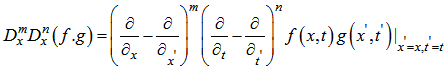 | (1.4) |
For example we have | (1.5) |
Though Hirotabi linear equations are special, there are many other differential equations which cannot be written in the Hirota bilinear form. In this paper, enlightened by the idea proposed in [9], we are going to investigate one of the several questions posed in the [9] I i. e mixing the DƤ-operators with different natural number Ƥ = 5 in order to formulate a more general bilinear equations so as to shed more light on the study of some kind of generalized bilinear differential operators and their corresponding bilinear equations, which have some nice mathematical properties. Another important issue we are also going to ascertain is the links between the bilinear equations and multivariate Bell exponential polynomial and their linear subspaces of solutions together with the linear superposition principle also as discussed in [9].
2. Bilinear Differential Equation Operators and Bilinear Equation
2.1. Bilinear 
In this section we will summarized the essential facts on bilinear differential operators and bilinear equations associated with the multivariate polynomial as given in [9]. Some definitions related to this may also be found in [10, 11]Let P be given a natural number. We introduce bilinear differential operators as follows: | (2.1) |
Where the powers of α are determined by  | (2.2) |
If p =1 the observe the normal derivative, while the cases of P = 2k, k є  , reduce to Hirota bilinear operators. (see, e. g [9] how the powers of α can be determined and the difference between the Hirota bilinear differential operator [1] and the Dp- operators).
2.2. Bilinear Equations
A bilinear differential equation associated with a multivariate polynomial [9]  is define by
 | (2.3) |
which reduces toHirota bilinear equation if  assuming p=3 we particularly have the generalized bilinear KdV equation
  The generalized bilinear Boussinesq equation
 | (2.4) |
and the generalized bilinear KP equation | (2.5) |
Such generalized bilinear equations have some common characteristics:Bilinear: the nearest neighbours to linear equations.In this paper, we also would like to discuss with more examples (other than that of [9]) that can also provide solution on:• How can one identify bilinear equations defined by (2.3)? and:• What type of exact solution are there to bilinear equation defined by (2.3)?through the Bell exponential polynomials and the linear superposition principle respectively。
3. Relations with Bell Exponential Polynomials
Let  be a sequence of real or complex numbers. Its partial (exponential) Bell polynomial
  is define as follows [10, 11]
 | (2.6) |
the exact expression can be written as | (2.7) |
Where the sum is over n-tuples of nonnegative integers  satisfying the constraint
3.1. Binary Bell Polynomials
Here also a summary of the main idea of the proposed work will be stated and some definitions regarding the Bell polynomials where two properties used to link bilinear equations to a special kind of Bell polynomials will be employed (see, for example [9] for the details). We first explore a relation of the Bell polynomials to the  -operators. For simplicity in the computational procedure we assume
  | (3.1) |
Thus using (work), we have 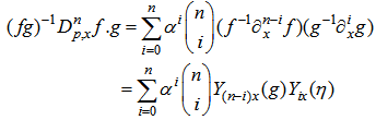 | (3.2) |
where  Similarly to the case of the Hirota D-operators [1], we introduce binary Bell
 | (3.4) |
Where  As an example we have
  | (3.5) |
Now setting  | (3.6) |
From (3.4), we have a combinatorial formula for the -operators | (3.7) |
We now introduce Ƥ-polynomials in order to qualify the bilinear equations | (3.8) |
The first few of the which in the case of Ƥ=5 read | (3.9) |
In terms of  | (3.10) |
The combinatorial formula (3.7) becomes | (3.11) |
if f= g, a relation between bilinear expressions and the  -polynomials will become
 | (3.12) |
Therefore the bilinear equation | (3.13) |
is equivalent to an equation and a linear combination of  -polynomials in
  :
: | (3.14) |
This is a characterization for our generalized bilinear equations in one dimensional case.
3.2. Multivariate Binary Bell Polynomials
For a  function
  , we can define the variables as in [9]
 | (3.15) |
and the multivariate Bell polynomials  | (3.16) |
which can be computed through  | (3.17) |
Three examples in differential polynomials function are  | (3.18) |
Based, on (3.16) we can show that the homogenous property  | (3.19) |
and the general Leibnitz rule | (3.20) |
implies the addition formula for the multivariate Bell polynomials : | (3.21) |
In a similarly manner [9] uses  | (3.22) |
for the sake of computational convenience and by (3.19) and (3.21) we can compute that | (3.23) |
Let us now introduce binary multivariable Bell polynomials in differential polynomials form: | (3.24) |
Where | (3.25) |
Then from (3.23) a combinational formula follows | (3.26) |
again on employing the following multivariable  -polynomials
 | (3.27) |
For example, we have  | (3.28) |
It now follows that | (3.29) |
Thus, a bilinear equation  | (3.30) |
is equivalent to an equation on a linear combination of multivariate Ƥ-polynomials in  | (3.31) |
where the coefficients  are constants. This is a characterization for generalized bilinear equations as discussed in [9], defined through the
  .
.
4. Linear Superposition Principle
4.1. Subspaces of Solutions
Let  be a multivariate polynomial. Consider a bilinear equation
 | (4.1) |
Define a set of N wave variables | (4.2) |
Where the are constants, and form a bilinear combination of N exponential waves
  | (4.3) |
Where all the  are arbitrary constantsNote that there are bilinear identities of the form
 | (4.4) |
Where the powers of α obey the rule (2.2). Following the criterion for obtaining the linear subspaces of solutions defined by [10] (see [5] and [6] for details) which stated a theorem that support an arbitrary linear combination of N exponential waves and an equivalent theorem on the linear subspaces of exponential N-wave solutions as in [7] we can use a type of parameterization for wave numbers and frequencies and list the sequential solution procedures as follows:We introduce of the independent variables: | (4.5) |
where the weight  can be both positive and negative.Form a homogenous polynomial
  defined by (3.30), in some weight.Parameterize
  using a parameter
  :
: | (4.6) |
and then determine the proportional constants  and the coefficients
  .
.
4.2. Illustrative Examples
In this section a few concrete examples will be given to illustrate the effectiveness of the approach.To present illustrative examples we consider the (2+1)-dimensional case with as again the (3+1)-dimensional case as presented in [9] | (4.7) |
and | (4.8) |
Then upon forming a homogeneous multivariate polynomial in some weight | (4.9) |
we solve the system (4.4) and (4.6) for the proportion constants  and the coefficients
  in order that the corresponding bilinear equation and their associated linear subspace of solutions consisting of linear combination of exponential waves we will be ascertained. We are now going to present two concrete illustrative examples by applying this general idea below in order to shed more light on the general ideaExample 1 Examples with positive weights let us set the weights of independent variables
  | (4.10) |
And consider a polynomial being homogenous in weight 4 | (4.11) |
Following the parameterization of wave numbers and frequencies in (4.8), we set the  | (4.12) |
Where  are the arbitrary constants but the proportional constants
  are to be determinedNow, a direct computation show that the corresponding bilinear equation reads
  | (4.13) |
The corresponding linear subspace of N-wave solutions is given by (4.14) | (4.14) |
where are arbitrary constants but the proportional constants are
  and are defined by
  | (4.15) |
Example 2 Example with positive and negative weightsLet us set weights of independent variables  | (4.16) |
and consider a polynomials being homogenous in weight 2 | (4.17) |
Following the parameterization of wave numbers and frequencies, we get the wave variables | (4.18) |
where  , are arbitrary constant but the proportional constant
  are to be determined by (4.5)Similarly, a similar direct computation shows that the corresponding bilinear equation reads
 | (4.19) |
and it possess the linear subspace of N-wave solutions determined by | (4.20) |
Where the  are arbitrary but
  need to satisfy
 | (4.21) |
5. Conclusions
We have discussed on the kind of the generalized bilinear differential operators  , their link with Bell polynomials and applied the linear superposition principle to the corresponding bilinear equations. We mixed the
  -operator with different natural number p = 5 to formulate a more general bilinear equation as it was posed for further investigation in [9].
References
| [1] | R. Hirota (2004) The direct method in soliton theory. Cambridge, Cambridge University, Press. |
| [2] | P.P Goldstein; Hints on the Hirota bilinear method, ACTA, Physicapolinica A 112 (6),(2007) 1-5. |
| [3] | R. Hirota; Exact solution of the KdV equation for multiple collisions of soliton. PhysLett. 27,(1971) 1192-1194. |
| [4] | R. Hirota; Exact N-soliton solution of wave equations of long wave on shallow water and in nonlinear lattices. J. Math. Phys. 14 (7)(1973) 810-814. |
| [5] | M. Y. Adamu and E. Suleiman; On the Generalized Bilinear Differential Equations, IOSR Journal of Mathematics 3, (4) (2012) 24-30. |
| [6] | M. Y. Adamuand E. Suleiman; On linear Superposition principle Applying to Hirota Bilinear Equations, American journal of computational and applied mathematics 3(1)(2013) 8-12. |
| [7] | W.X. Ma, J.-H. Lee; A transformed rational function method and exact solutions to the 3+1 dimensional Jimbo–Miwa equation, Chaos Solitons Fractals42 (2009) 1356–1363. |
| [8] | A.M. Wazwaz; Multiple-soliton solutions for a(3+1)-dimensional generalized KP equation, Commun.Nonlinear Sci. Numer.Simul. 17 (2012) 491–495. |
| [9] | Wen-Xiu Ma; Bilinear equation, Bell polynomials and linear superposition principle; J. of Phy. (411) 2013. |
| [10] | SadekBouroubi, Moncef Abbas: New identities for complete Bell polynomials based on formula of Ramanujan . J. of int. Seq. (12); 2009 #p34. |
| [11] | Daniel Birmajer, Juan B. Gil Michael D. Weiner; Some Convolution identities and an inverserelation involving partial Bell polynomialsthe electronic journal of combinatorics 19(4) (2012). |
| [12] | W.X. Ma, T.W. Huang, Y. Zhang; A multiple exp-function method for nonlinear differential equations and its application, Phys. Scr. 82 (2010) 065003. |
 Abstract
 Reference
 Full-Text PDF
 Full-text HTML