1. Introduction

The mass transfer in laminar boundary layer flow over a moving surface in porous medium has many important applications in modern industry. Thus the boundary layer flow problems have been widely studied over the past few decades and the earlier investigators were interested in finding the similarity solutions for the boundary layer flow problems, viz. Blasius [1], Howarth [2], Sakiadis [3], Siekman [4], Klemp [5] and Abussita [6].

For the boundary layer flow on a moving flat plate in a quiescent fluid, Sakiadis [3] obtained the same equations as obtained by Blasius [1] with different boundary conditions. Abdulhafez [7] and Hussaini et al. [8] reported the fluid flow characteristics for moving wall laminar boundary layer problems. Similar problems with various boundary conditions and in different situations have been considered by Lin [9], Weidman et al. [10] and Cortell [11]. Ishak [12] extended the classical problems of Blasius [1] by considering a flat plate moving in the same or opposite directions to a parallel free stream, all with constant velocities. Heat transfer in a moving fluid over a moving non-isothermal flat surface is investigated numerically by Mukhopadhyay [13] and dual solutions for boundary flow of moving fluid over a moving surface with power–law surface temperature is studied by Mukhopadhyay and Gorla [14]. By introducing composite velocity, Afzal et al. [15] combined Blasius and Sakiadis problems successfully and obtained a single set of equations.

Andersson [16] investigated the transport of mass and momentum of chemically reactive species in the laminar flow over a linearly stretching surface and solved the nonlinear ordinary differential equations governing the self-similar flow. Takhar et al. [17] studied the flow and mass diffusion of chemical species with first and higher order reactions over a continuously stretching sheet with an applied magnetic field. Uddin M.S. [18] studied the boundary layer flow and reactive solute transfer with first order reaction past a stretching surface, the variable initial solute distribution along the surface is taken into account.

Bhattacharyya [19] investigated the mass transfer with first order chemical reaction on a continuous flat plate moving with constant velocity in parallel or reversely to a uniform free stream; the variable reaction rate is considered. Merkin [21] studied dual solution through porous medium, while mass transfer over permeable surface is investigated by Magyari [22]. Elbashbeshy and Bazid [23] studied the mixed convection along a vertical plate with variable surface heat flux embedded in porous medium.

Nabil T. M. Eldabe et al [24] studied the effects of chemical reaction and fluid flow through a porous medium over a horizontal stretching flat plate. The boundary layer flow and mass transfer over a stretching sheet embedded in porous medium is investigated by Hossen [25].

Elbashbeshy and Sedki [26] studied the effect of chemical reaction on mass transfer over a stretching surface embedded in a porous medium.

The aim of the present study is to investigate the effects of chemical reaction and diffusion in boundary layer flow with mass transfer over permeable flat plate moving reversely or parallel to a free stream of a moving fluid embedded in porous medium. In this analysis, the wall concentration is variable. The present study may be regarded as an extension to Ishak [12]. The numerical computations are carried out for several values of parameters involved in the transformed equations viz. the suction or injection parameter (s), the Schmidt number (Sc), the chemical reaction rate parameter (B), the power –law exponent (n), Porous parameter (N) and the velocity ratio parameter (q). The features of the flow and mass transfer characteristics viz. variation of a velocity profiles velocity , Variation of a skin friction coefficient , Concentration profiles φ (η) and concentration gradient at the surface φ′ (0) for different values of the governing parameters are discussed and analyzed.

2. The Governing Equations

We consider the two-dimensional steady laminar boundary-layer flow of an incompressible, viscous fluid and mass diffusion with chemical reaction over a flat surface subject to suction or injection with variable wall concentration. The surface moves with constant velocity U_w in the same or opposite direction to the free stream embedded in porous medium. The x -axis extends parallel to the surface, while the y -axis extends upwards, normal to the surface. Using boundary layer approximation, the governing equations for the flow and concentration distribution may be written as

(1)

(2)

(3)

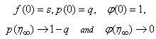
Where (x, y) are the dimensional coordinates along and normal to the tangent of the surface and (u, v) are the velocity components parallel to (x, y). is the kinematic viscosity where ρ is the density and is the dynamic viscosity of the fluid. C is the concentration, D is the diffusion coefficient and C₀ is the concentration in the free stream. R(x) is the variable reaction rate of the solute and is given as , L is the reference length and R₀ is constant.

The boundary conditions for the velocity components and the concentration are

(4)

(5)

Where the free stream velocity is is the variable plate concentration and C₀ is a positive solute constant. n is a power-law exponent which signifies the change of amount of solute in the x-direction. is the variable suction or injection through the permeable plate and is given by , is a constant with for suction and for injection.

The stream function ψ (x, y) that satisfies the continuity equation and is related to the velocity components in the usual way as

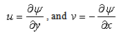(6)

Using boundary layer approximation, the following dimensionless variables for ψ and C can be introduced

(7)

then we have

(8)

(9)

(10)

(11)

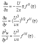
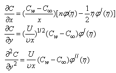
Where is the local Reynolds number and ƞ is the similarity variable defined as where U is the composite velocity defined as U=U_∞+U_w (Afzal et al. [15]). is the dimensionless stream function and φ is the dimensionless concentration function. Substituting in equations (6-9) to obtain the set of ordinary differential equations

(12)

(13)

Where is the porous parameter, is the Schmidt number and is the chemical reaction rate number. The boundary conditions finally become

(14)

(15)

Where the velocity ratio parameter q = u_w /U and s is the suction or injection parameter where

,

S > 0 ( i.e. < 0) corresponds to suction and S < 0 (i.e. > 0 ) corresponds to injection. The physical quantities of interest in this problem are the local skin-friction coefficient and rate of mass transfer - which are defined as

(16)

(17)

3. Numerical Method of Solution

The system of the nonlinear ordinary differential equations (12-13) along with the boundary conditions (14-15) is solved by using the following methods

(1) Fourth order Rung Kutta Method (RKM)

(2) Keller Box Method (KBM)

3.1. Fourth Order Rung Kutta Method (RKM)

The numerical method (RKM) is based on fourth order Runge-Kutta iteration scheme with shooting method [19]. The system (12-15) is solved by RKM, by converting it into an initial value problem. In this method we have to choose a suitable finite value of , say .

We set the following first order system:

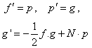(18)

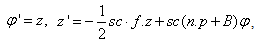(19)

With the boundary conditions

(20)

To solve the system of the initial value problem (18 -19) with (20) we need values for and but no such values are given in the boundary conditions. The initial guess values for and are chosen and applying fourth order Runge –Kutta method then solution is obtained. To get accurate solution, it is important for shooting method to choose the appropriate finite value of . In order to determine for the initial value problem (18-20), we start with some initial guess values for some particular set of the physical parameters to obtain and . The solution procedure is repeated with another value of until two successive values of and differ only by the specified significant digit. The last value of is finally chosen to be the most appropriate value of the limit for that particular set of parameters. The value of may change for another set of physical parameters. After determining the value , we compare the calculated values of and at with the given boundary conditions and and adjust the values of and using Secant method to give better approximation for the solution. The step size is taken as . The process is repeated until we get the results correct up to the desired accuracy 10^-6 level.

3.2. Keller Box Method (KBM)

The system of the nonlinear ordinary differential equations (12-15) is solved numerically by Keller-Box method [27, 28] that is an implicit finite difference method. One of the basic ideas of the Keller-box method is to write the governing system of equations in the form of a first order system (18-20). We use centered – difference derivatives and averages at the midpoint of net rectangles to get finite difference equations with a second order truncation error. The method allows for non-uniform grid discretion and converts the differential equations into algebraic ones that are then solved using Thomas algorithm. Thomas algorithm is essentially the result of applying Gauss elimination to the tri-diagonal system of equations. The number of grid points in both directions affects the numerical results. To obtain accurate results, a mesh sensitivity study was performed.

3.2.1. The Finite-Difference Scheme

We now consider the net rectangle in the plane and the net points defined as follows:

where is the - spacing and is the -spacing. Here i and j are just sequence of numbers that indicate the coordinate location, not tensor indices or exponents. The derivatives in the -direction are replaced by finite difference, for example the finite- difference form for any points are

,

We start by writing the finite difference of equations for the midpoint using centered –difference derivatives, we get

If we assume , , , , to be known for , then we have to obtain the solution of the unknown (,, ,, ) for . The system can be written as

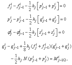(21a)

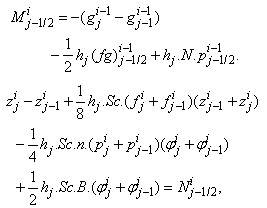where

where

We note that and involves only known quantities if we assume that the solution is known on . The transformed boundary layer thickness is to sufficiently large so that it is beyond the edge of the boundary layer [29, 30]. The boundary conditions at yields

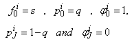(21b)

3.2.2. Newton‘s Method

To linearize the nonlinear system of equations using Newton’s method, we introduce the following iterates

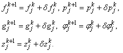After dropping the quadratic and higher order terms in , and . We have also dropped the superscript (k) for simplicity. This procedure yields the following linear tri-diagonal system.

(22a)

where

To complete the system (22a), we recall the boundary condition (21b), which can be satisfied exactly with no iteration. So, to maintain these correct values in all the iterates, we take

(22b)

3.2.3. The Block Tri-diagonal Matrix

The linearized difference equations (22) has a block tri-diagonal structure consists of variables or constants, but here it consists of block matrices. The elements of the matrices are defined as follows,

That is:

(23)

,

To solve the system (23), we assume that A is nonsingular and can factorized into , where

Now we have ,

if we define

(24)

then we have

(25)

the elements can be solved from equation (25)

Where the step in which , and are calculated, is usually referred to as the forward sweep. Once the elements of are found, equation (24) then gives the solution in the so called backward sweep, in which the elements are obtained by the following relations:

these calculations are repeated until some convergence criterion is satisfied and calculations are stopped when , where is small prescribed value.

4. Results and Discussion

The nonlinear system of differential equations (18-20) is solved numerically by both Keller-Box method which is an implicit finite difference method and also by the numerical method based on fourth order Runge-Kutta iteration scheme with shooting method and the computer programming methods are done in MATLAB. For the confirmation of the accuracy of applied numerical methods we compare our results corresponding to the values of numerically obtained skin-friction coefficient for various of q with previously reported by Ishak [12] and excellent agreement are found for the used numerical methods as shown in Table 1. The numerical computations are carried out for several values of parameters involved in the equations viz. the suction or injection parameter (s), the Schmidt number (sc), the chemical reaction rate parameter (B), the power –law exponent (n), porous parameter (N) and the velocity ratio parameter (q).

Table 1. Skin-friction coefficient       for various of q with N=0 and S=0

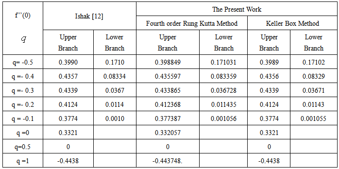
The computed results are explained by plotting some figures for variation of a velocity profiles , Variation a skin friction coefficient , Concentration profiles φ(η) and concentration gradient at the surface φ′(0) for different values of the each parameter and physical meaning are also given.

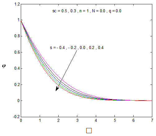
The external suction or injection parameter (S) effects are demonstrated in Figures (1-6), it is found that at fixed ,variation of a velocity profiles and variation of a skin friction coefficient increase with the increase of the suction (S) while both Concentration profiles φ(η) and concentration gradient at the surface φ′(0) reduce. It is due to the fact that the momentum as well as concentration boundary layer thicknesses decrease with suction.

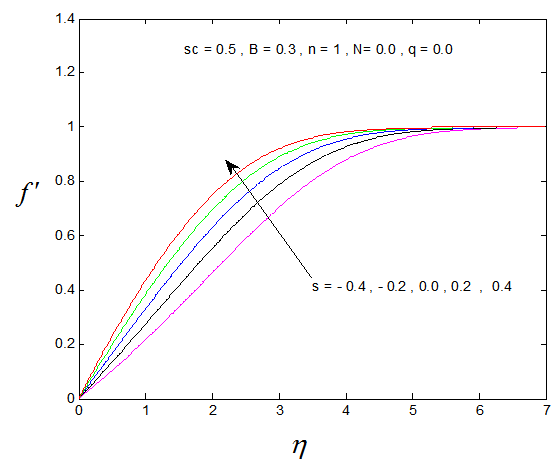Figure 1. for different values of s

Figure 2. for different values of s

Figure 3. against for different values of s

Figure 4. for different values of s

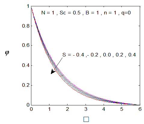Figure 5. φ(η) for various values of s

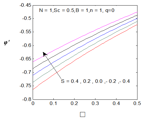Figure 6. φ′ (0) for different values of s

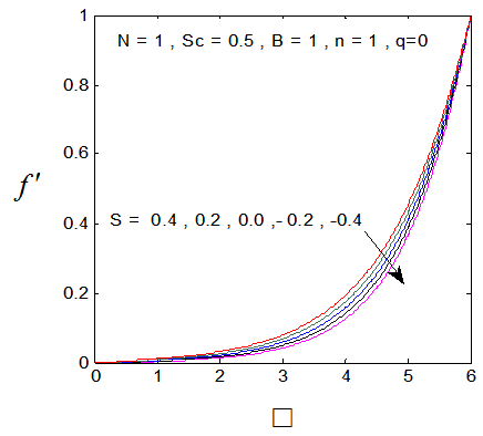
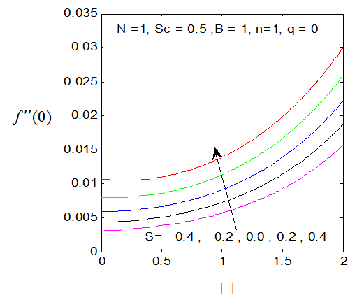
On the other hand for the external injection case, with the increasing injection, variation of a velocity profiles and variation of a skin friction coefficient decrease and Concentration profiles φ (η) and concentration gradient at the surface φ′ (0) increase. It is due to the injection, both momentum and boundary layer thicknesses increase.

The Schmidt number (Sc) effects are displayed in Figures (7-8), it is observed that The Schmidt number has major effects on the distribution of solute. At fixed ƞ the increase of Schmidt Sc reduces quickly both concentration profiles φ(η) and concentration gradient at the surface φ′(0). This is due to the fact that the rate of solute transfer from the surface increases when the Schmidt number increases. The negative value of the concentration profile for large Sc is because of substantial increase in the rate of solute transfer from the plate to the fluid in the chemical reaction. It is observed that the magnitude of the concentration gradient initially increases with Sc, but for greater values of it decreases with Sc.

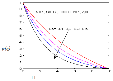Figure 7. φ (η) for various values of Sc

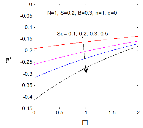Figure 8. φ′ (0) for different values of sc

The effects of the reaction rate parameter (B) are illustrated in Figures (9-10), it is found that the reaction rate parameter affects the solute profiles in similar way as that of the Schmidt number i.e., the increase of the reaction rate parameter B at fixed reduces both the concentration profiles φ (η) and concentration gradient at the surface φ′(0) and thus the chemical reaction enhances the mass transfer.

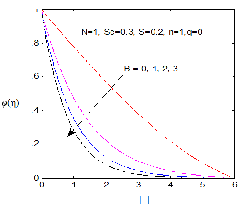Figure 9. φ(η) for various values of B

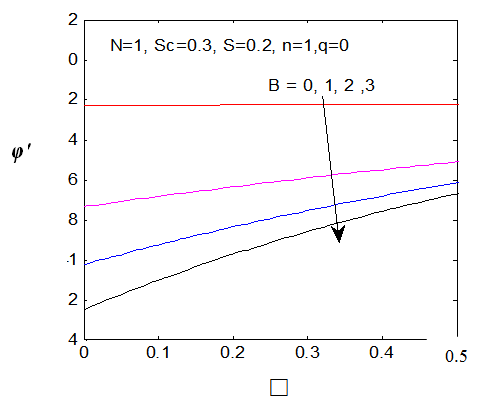Figure 10. φ′(0) for different values of B

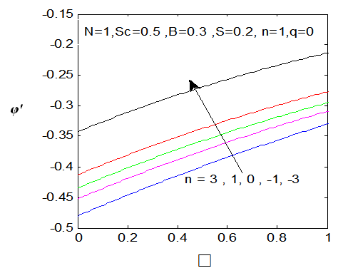
The effects of the power –law exponent (n) are shown in Figures (11-12), it is observed that the increase of the power –law exponent n with n > 0 reduces Concentration profiles φ (η) at fixed . While the concentration profile increases with the increase in the magnitude of n with n < 0 and for large negative values of n, the overshoot of solute is observed near the surface. The magnitude of the concentration gradient at the surface φ′ (0) increases with the increase in positive n but decreases with the increase in the magnitude of n. with n < 0. Thus, the effect of increase of n when the surface concentration is which is completely opposite to the effect of the increase of n when the surface concentration is . Note that, the wall concentration is constant when n=0.

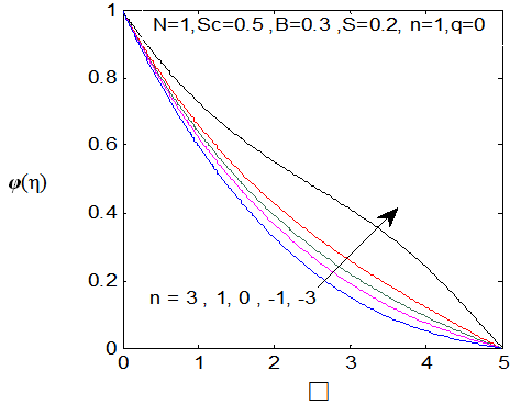Figure 11. φ(η) for various values of n

Figure 12. φ′(0) for different values of n

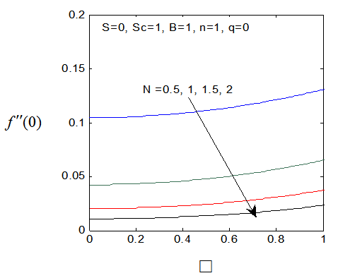
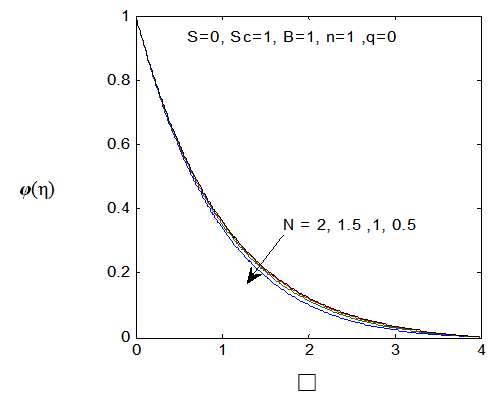
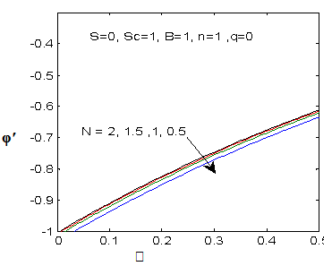
Porous parameter (N) effects are demonstrated in Figures (13-16), it is found that at fixed , variation of a velocity profiles and variation of a skin friction coefficient decrease with the increase in porous parameter while the increase of N increase both concentration profiles φ(η) and concentration gradient at the surface φ′(0). Also it is shown in Figures (1-3, 5, 13) that the presence of a porous medium increases the resistance to flow resulting in decrease in the flow velocity and increase in the solute concentration which increases the solute boundary layer thickness.

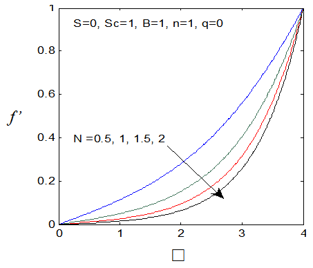Figure 13. for different values of N

Figure 14. for different values of N

Figure 15. φ(η) for various values of N

Figure 16. φ′(0) for different values of N

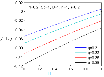
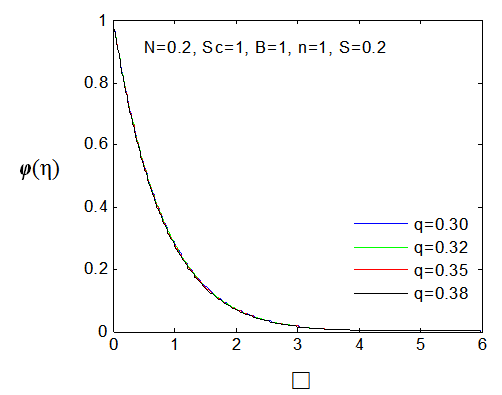
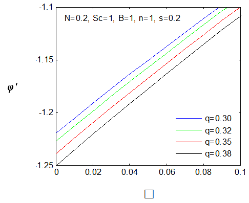
The velocity ratio parameter (q) effects are illustrated in Figures (17-20), it is observed that at fixed , variation of a skin friction coefficient decreases with the increasing in q > 0 while variation of a velocity profiles increases but far away from the plate decreases. The increase of q > 0 reduce both concentration profiles φ(η) and concentration gradient at the surface φ′(0).

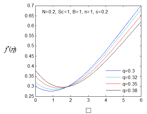Figure 17. for different values of q

Figure 18. for different values of q

Figure 19. φ(η) for various values of q

Figure 20. φ′(0) for different values of q

It is seen in Figures (21-22) that the solution are unique when q > 0, while dual solutions are found to exist when q < 0, i.e. when the plate and the free stream move in the opposite directions. it is noticed in Figure (21) that the momentum boundary layer thickness increases in the upper branch solution with the increasing of the magnitude of the velocity ratio parameter and for the lower branch solution it decreases with magnitude of q. 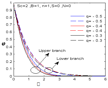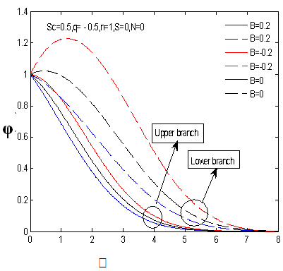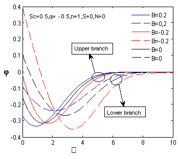The concentration φ(η) at Figure 22 increases with magnitude of q for the upper branch in any point and for the lower branch solution initially increases with magnitude of q and for large changing the nature, it decreases. It is shown in table (1) that the values of f ′′(0) are positive when q < 0.5, and they become negative when the value of q exceeds 0.5. The concentration profiles φ(η) and concentration gradient φ′(0) for some values of the chemical reaction rate parameter (B) are presented in Figures 23 and 24 respectively. These profiles satisfy the boundary conditions (13), which support the numerical results besides supporting the dual nature of the solutions presented in Figures (21-23). They show that φ(η) increases for both solutions with the decreasing of B in any point while Figure 24 shows that the concentration gradient φ′(η) for both solutions initially decreases with the increasing of B but far away from the plate it increases.

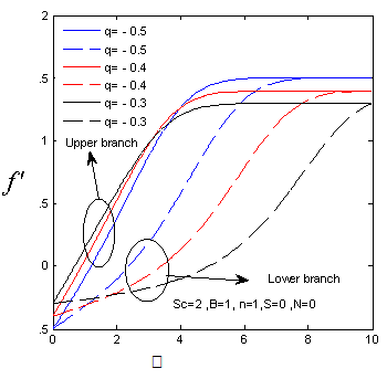Figure 21. for different negative values of q

Figure 22. for different negative values of q

Figure 23. for different negative values of B

Figure 24. for different negative values of B

5. Conclusions

The development of boundary layer flow with mass transfer through porous medium over a moving permeable flat plate with variable wall concentration in the presence of first order chemical reaction is investigated. The classical Blasius (1908) and Sakiadis (1961) problems are particular cases of the present problem. Also Ishak (2007) is extended by the present work. The nonlinear system of nonlinear differential governing equations is solved numerically by both Keller-Box method and the method based on fourth order Runge-Kutta iteration scheme with shooting method. A comparison is made with particular case of the present study previously reported by Ishak [12] and the results are found to be in excellent agreement. We found that, the Variation of a velocity profiles and variation of a skin friction coefficient decrease with the increasing in porous parameter N while both concentration profiles φ(η) and concentration gradient at the surface φ′(0) increase. The increasing of the velocity ratio parameter (q), suction or injection parameter S, the reaction rate parameter B , the Schmidt number Sc and the power–law exponent (n) reduce both Concentration profiles φ(η) and concentration gradient at the surface φ′(0). The increasing of velocity ratio parameter (q) increases the variation of a velocity profiles but far away from the plate it decreases. Dual solutions are found to exist when q < 0 i.e. the plate and the free stream move in the opposite directions. Consequently, the solute boundary layer thickness is found to increase with the increase of magnitude of q for the upper branch and in the lower branch it decreases. It is found that both φ(η) and the concentration gradient φ′(η) increase for dual solutions with the decreasing of B in any point but far away from the plate the concentration gradient φ′(η) decreases for dual solutions.