1. Introduction

Buruli ulcer is a debilitating human skin disease caused by Mycobacterium ulcerous [16].This infection is a neglected emerging disease that has recently been reported in some countries as the second most frequent mycobacterial disease in human tuberculosis [1]. A large number of lesions often result in scarring, contractual deformities amputations and disabilities [3]. In Africa, all ages and sexes are affected, but most cases of the disease occur in children between the ages of 4-15years [6]. It has emerged dramatically over the past two decades especially in Central and West Africa and has been confirmed by laboratory tests in 26 countries with reports in other countries around the world [2, 4]. Burului ulcer has been reported in over 30 countries mainly with tropical and subtropical climates but it may also occur in the same countries where it has not yet been recognized such as Burkina Faso and Guinea [2]. Notable contributing factors for Buruli ulcer outbreak include deforestation, eutrophication, dam construction, farming and habitat fragmentation. When treatments are delayed often in West Africa where due to lack of adequate knowledge about the disease they normally reported late, infections could lead to ulcerated lesions[16].When data from Ghana were analysed it was revealed that socioeconomic impact had a huge economic burden on affected countries. For example, gross domestic product per capital (Ghana) in 1998 was estimated at USD 399.41. The cost of surgical excisions of a large ulcer including 3 months inpatient expenses, transportation, food and income lost was USD 783. The current strategy of controlling the disease includes the use of drugs, surgery, heat, hyperbaric oxygen and traditional medicine. These are strong social economic ways to the burden of the BU disease, which in different ways affects fertility, population growth, saving and investment, absenteeism, stigmatization of women in adulthood for marriage and medical cost [19].

Modeling of epidemiological phenomena has a very long story with the first model for smallpox formulated by Daniel Bernoulli in 1760. Mathematical modeling of the population models continues to provide vital insights into population behaviour and control. In the past years this has become an essential tool in understanding the dynamics of diseases, and the decision which has to do with process regarding intervention programs for controlling population and disease problems and in many countries. Similarly, different techniques have been employed to study vital optimal control problem related to dynamical systems. In particular, [10] developed a continuous model for malaria vector control with the objective of studying how genetically modified mosquitoes should be introduced in the environment using optimal control problem strategies. [13] applied optimal control theory to model malaria disease that includes treatment and vaccination with warning immaturity, to study the impact of a possible vaccination with treatment strategies in controlling the spread of malaria. Time- -depend-control strategies have been applied for the study of HIV model [11, 12] for strain tuberculosis models. [14] also examined SIR epidemiological models numerically and obtains controls that exert maximum efforts on some initial interval.

To the best of our knowledge there is no single mathematical model available with optimal control theory application on BU diseases. In this study, we desire and analyze a Buruli ulcer disease transmission mathematical model. We study and determine the possible impact of optimal treatment and preventing on the spread of Buruli ulcer. Theoretically, we analyzed the stability properties. We also undertake a detailed qualitative optimal control analysis of the resulting model, and we determine the necessary conditions for optimal control of the disease using Pontryagins Maximum Principle in order to obtain optimal strategies for controlling the spread of the disease. The aim of this paper is to develop an optimal control that minimizes the number of Burului ulcer infected hosts, vector and fish with optimal cost of mass treatment and insecticides using Pontryagins Maximum Principle.

This paper is arranged as follows; in Section 2, we formulate and establish the basic properties of the model. The steady states are determined and analysed for their stability in Section 3. Parameter estimation and sensitivity analysis are given in Section 4. Numerical results on the behavior of the model are also presented in this section. In Section 5 we present the application of the model to a real life situation and concluded in Section 6.

2. The Model and Its Analysis

2.1. Model Formulation

Based on the described transmission dynamics of Buruli ulcer, we formulate a constant human population N_H(t), the vector population of water bugs N_V (t) and the fish population N_F(t) at any time t. We consider SIR model for human population and SI model for both water bugs (vector) and fish .The total human population is divided into three epidemiological subclasses of those that are susceptible S_H(t), the infected I_H(t) and the recovered R_H(t). Total population of vector (water bug) at any time t is divided into two subclasses to susceptible water bugs S_V (t) and those that are infectious and can transmit the buruli ulcer to humans, I_V (t). The total population reservoir of small fish is also divided into two compartments of susceptible fish S_F(t) and infected fish I_F(t). We also take into account the role played by environment and therefore introducing a compartment U, denoting the density of Mycobacterium ulcerans in the environment. We make the following basic assumptions:

● Mycobacterium ulcerans is transferred only from vector ( water bug) to humans.

● There is homogeneity of human, water bug and fish populations interactions.

● Infected humans recover and can be re-infected with Mycobacterium ulcerans again. We thus have loss of immunity.

● Fish are preyed on by the water bugs.

● Susceptible host (human population) can be infected through biting by an infectious vector (water bug). We represent the effective biting rate that an infectious vector has to susceptible host as β_H and the incidence of new infections transmitted by water bugs is expressed by standard incidence rate . One can interpret β_H as the product of the biting frequency of the water bugs on humans, density of water bugs per human host and the probability that a bite will result in an infection.

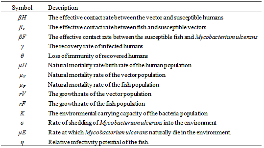
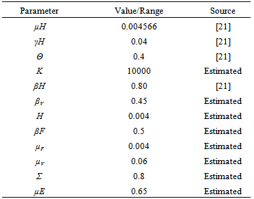
● Susceptible water bugs are infected at a rate through predation of infected fish and representing other sources in the environment. Here η differentiates the infectivity potential of the fish from that of the environment.

● The vector population and the fish populations are assumed to be constant. The growth functions are respectively given by g(N_V ) and g(N_F). Without loss of generality, we can assume that the growth functions are given by

g(N_V) = µ_V N_V and g(N_F) = µ_FN_F.

It is important to note that logistic functions can be chosen as growth functions for richer dynamics. In this work, we however assume that the growth functions are linear.

● There is a proposed hypothesis that environmental mycobacteria in the bottoms of swamps may be mechanically concentrated by small water-filtering organisms such as microphagous fish, snails, mosquito larvae, small crustaceans, and protozoa [5]. We thus assume that fish increase the environmental concentrations of Mycobacterium ulcerans at a rate σ.

● The model does not include a potential route of direct contact with the bacterium in water.

● The birth rate of the human population is directly proportional to the size of the human population.

The possible interrelations between humans, the water bug and fish are represented by the schematic diagram below.

The descriptions of the parameters that describe the flow rates between compartments are given in Table 1.

Table 1. Description of parameters used in the model

Considering the assumptions made above, the interaction among humans, water bugs (vector), small fish population and MU in the environment, the dynamics of Buruli ulcer can be described by the following set of nonlinear differential equations:

(1)

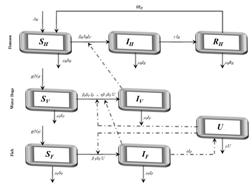Figure 1. Proposed transmission dynamics of the Buruli ulcer among fish, the water bug and humans

We assume that all the model parameter are positive and the initial conditions of the model system (1) are stated as

.

The region of biological interest of model (1) is

and

where is constant.

We note that model (1) is well positioned in the non-negative region for the fact that the vector and fish as well as the environment do not point to the exterior. By providing an initial condition in the region, then we can define solution for all time and remains in the region.

2.2. Positivity of the Solution

We show that for any non-negative initial conditions of the system (1), the solutions still remain non-negative for all. We desire to prove that all necessary state variables in the system (1) remain non-negative and also the solutions of the system with positive initial conditions will stay positive for all . We therefore, propose the following lemma.

Lemma 1. Given that the initial conditions of the system (1) are positive, the solutions ,,,,, , and are non-negative for all

Proof. Given that

.

More precisely , and it implies directly from the first equation of the system (1) that

where.

We therefore have

.

Thus

and that

The right hand of (3) is obviously positive. Therefore, the solution will at any given instance be positive.

In examining the second equation of 1,

Similarly, it can be determined that ,,,,, and for all , and this leads to the completion of the proof.

3. Steady States and the Model Reproduction Number

In this section, We compute the equilibrium points by equating the right side of model (1) to zero. This direct computation indicates that model (1) always possesses a disease free equilibrium point where and a unique endemic equilibrium in Ω where

3.1. The Model Reproduction Number

Basic reproduction ratio is the expected numbers of secondary cases of infection per primary case of infection in a virgin population during the infectious period of primary case [17]. By applying the next generation operator approach [18], we represent F and V respectively as matrices for the new infections generated and the transition terms we get

and

The basic reproduction number ℜ₀ is expressed as the spectral radius of the matrix FV⁻¹ and therefore . The model reproduction number is determined by fish population and the density of Mycobacterium ulcerans in the environment. The reproduction number of the model (1) appears to be in ascendancy linearly with shedding rate of MU into the environment and effective contact rate between fish and MU. The spread of BU from model (1) does not depend on humans and the vector.

3.2. Stability of the Disease Free Equilibrium

Theorem 1. The disease free equilibrium whenever it exists is locally asymptotically stable if and unstable otherwise

The Jacobian matrix of model (1) at the equilibrium point E₀ is expressed by

It can be observed that the eigenvalues of are (µ_H + γ),(σ + µ_H),−µ_F,−µ_H,−µ_V ,−µ_V and the roots of quadratic equation . The computational results of Q(λ) = 0 shows to have negative parts only if . We can therefore make a conclusion that the disease free equilibrium is locally asymptotically stable whenever .

3.3. Stability of the Endemic Equilibrium

We examine the local geometric characteristics of the endemic equilibrium of model (1). We state the following theorem:

Theorem 2. If the endemic equilibrium point model (1), is locally asymptotically stable.

However, it is difficult to deal with stability of endemic equilibrium analytically because it contains a quadratic equation. By numerical approach, the endemic equilibrium is locally asymptotically stable. This is depicted in 2. We apply three different initial conditions for the simulation. Those orbits shown to be the same point as time evolve.

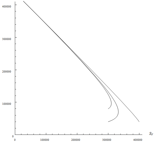Figure 2. Shows phase potrait of model (1) in SV — IV plane

4. Analysis of Optimal Control

Our state system is the following system of eight ordinary differential equations

(2)

The control where , deals with reducing the exposure of susceptible humans to those infected water bugs. This can be achieved by using insecticides and preventing the exposure of the human body from biting by water bugs. The control , models the efforts needed in bringing down the infection the water bugs and fishes. The last control examines the efforts required in reducing the infection between the water bugs and the environment. In order to achieve a successful control of BU, the effort is needed in the determination of the infected and also strictly putting measures to reduce it.

The objective is to minimize the number of infected humans in a settlement while maintaining the cost associated to control , and as much as possible. Therefore, we seek to minimize the number of Buruli ulcer infected hosts and cost of employing mass treatment, insecticide controls and reducing the number of infected fishes. Our optimal control problem with objectives function is expressed as

(4)

where , and are the weighting constants for the mass treatment human host, insecticide activities and mass treatment for infectious fishes are nonlinear and are of quadratic forms.

We therefore, seek an optimal control and such that

(4)

where

,

We analyze model 3, in other words model of the spread of Buruli ulcer in population applying optimal perspective. We take into account the objective function 4 to model 3. Pontryagins Maximum Principle will be employed to determine the optimal control and with necessary conditions. The necessary conditions to establish optimal control and that meet condition 5 and its constraint model 3 will be determined by applying Pontryagins Maximum Principle (Pontryagin). The principle changes (3), 4 and 5 into a problem of minimizing pointwise a Hamiltonian, H, with respect to , simply

where is the right hand side of the differential equations of the ith state variable. By using Pontryagin’s Maximum Principle and the existence of results obtained for optimal control, we achieve

Theorem 3. There exists an optimal control and corresponding solution, and , that minimizes over . Furthermore, there exist adjoint functions, , such that

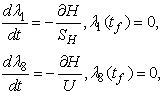
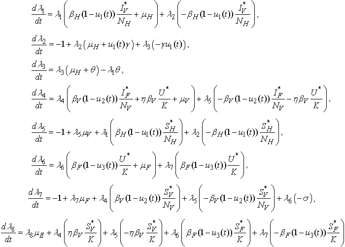(6)

with transversality conditions

(7)

and ,,,

Theorem 4. The optimal control that minimizes over is expressed as

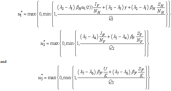(8)

Proof. [7] provides the existence of an optimal control due to the convexity of integrand with respect to (), a priori boundedness of the state solutions, and the Lipschitz property of the state system with respect to the state variables. Employing Pontryagin’s Maximum Principle, we have

(9)

Computed at the optimal control pair and respective corresponding states, which leads to the stated adjoint system (6) and (7), [22]. By taking into account the optimality conditions,

And determine the values for subject to the constraints, the characterizations (8) can be obtained. We illustrate the characterization of , we obtain

By considering the bounds on, we have the characteristics of in 8. By the fact that there is a priori boundedness of the state and adjoint functions and the resulting Lipschitz structure of the ODEs, we get the uniqueness of the optimal control for small value of t_f. The uniqueness of the optimal control based on the uniqueness of the optimality system, which is made up of 3 and 6, 7 with characterization 8. In order to guarantee the uniqueness of the optimal system, we put a restriction on the length of the time interval. The restriction on the length of time is as a result of opposite orientation of 3, 6 and 7. The stated problem contains the initial values and the adjoint problem contains final values.

5. Numerical Results

In this section, we study numerically an optimal treatment strategy of our Buruli ulcer dynamics model. We solve the optimal control problem using an iterative scheme derived by [24].

Table 2. Parameter values used for the simulations

The optimal strategy is obtained by solving the optimally system, made up of 16 ODEs from the state and adjoint equations. We begin by solving the state equations with a guess for the controls on the simulated time applying a forward fourth order Runge- Kutta scheme. By the fact that we have transversality conditions 7, the adjoint equations are overcome by a backward fourth order Runge- Kutta scheme applying the immediate iteration solution of the state equations. There after, the controls are updated by employing a convex combination of the previous controls and value obtained with respect to characterizations 8. The process is repeated and stopped if the values of unknowns at the formal iteration are very close to the ones at the current iteration [20]. In order to present numerical simulations, we use parameter values as in 2, and our initial condition y(0) = (400,40,100,100,20,100,10,10) and the weighting control is stated as Q₁ = 50,Q₂ = 20,Q₃ = 30 . We assume the weighting factor Q₁ in connection with mass treatment control u^∗₁ is greater than Q₂ and Q₃ which is associated with insecticide and mass public education respectively. The cost of mass treatment includes the cost of screening, cost of medications, and expenditure on the person taking care of the BU patient. Cost of insecticide also includes the cost of machines for spraying and labour cost and the cost of transportation of the personnel and chemicals. With regard to mass public education, the cost involved includes the cost of labour, cost of transportation, cost of manual materials. With respect to time horizon, we use 100 days.

5.1. Mass Treatment Control

In this section, we consider only control on mass treatment and both control and are set zero. The profile of the optimal control is depicted in Figure 5.1 (a). In order to do away with Buruli ulcer disease in 100 days, the treatment should be held intensively almost 100 days. By applying optimal control in Figure 5.1(a), we show the dynamics of infected humans, water bug, small fishes and Mycobacterium in the environment as observed in Figure 5.1(b, c,d, e) respectively. These numbers increase without optimal control and that is to say if there is no mass treatment. It is interesting to observe from Figure 5.1 (c) that without the mass treatment the number of infected water bug decreases. However, the addition of this control increases the rate of the reduction of the infection and slows the reduction otherwise.

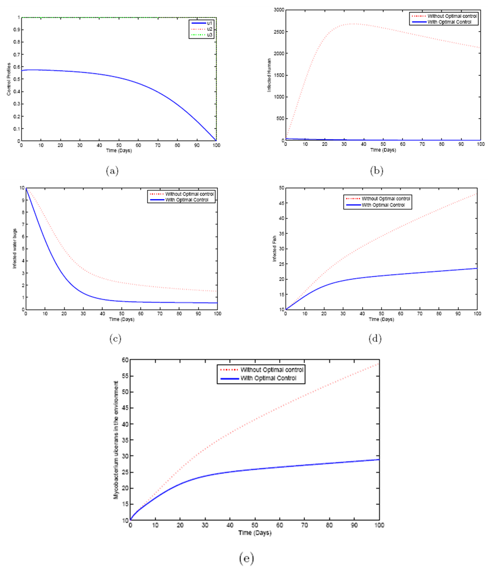Figure 5.1. Shows the profile of the optimal control u1 and optimal solution for infected humans, water bugs, small fish and MU in environment via mass treatment only

5.2. Insecticide Control

In this regard, we set both mass treatment control and mass education control we then activate only which is the insecticide as shown in Figure 5.2 (a). We show the profile of the optimal control on insecticide (Figure 5.2(a)). It is observed in Figure 5.2 (b) that the number of infected humans drastically decreases with the application of insecticide control. This situation reverses without the control . In Figure 5.2 (c), the infected water bug reduces without the control but with the control the reduction is higher. This process reduces without the application of insecticide. Figure 5.2 (d) depicts that infected small fish reduces with insecticide control and increases without the control . We also observed in Figure 5.2(e) that the shedding of MU in the environment decreases with insecticide control and increases in the environment without the control. That is to say, increase in shedding of MU in the environment.

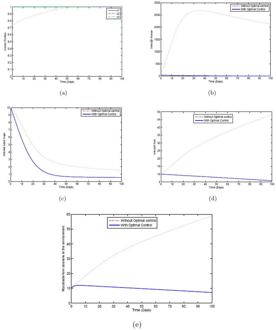Figure 5.2. Shows the profile of the optimal control u2 and optimal solution for infected humans,water bugs, small fish and MU in environment 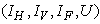via insecticide application only

5.3. Mass Education

In this scenario, we activate only the control on mass education while both controls and are set to zero. Figure 5.3 (a) depicts optimal control . In order to eliminate BU in 100 days, the mass education must be carried out intensively for almost 100 days as observed in Figure 5.3(a). In Figure 5.3 (b), the number of infected humans decreases drastically with control . That is to say, mass education and situation increase without mass education control . Interestingly, in Figure 5.3 (c) infected water bugs decreases sharply with mass education which is control and infected water bugs increase otherwise. Figure 5(d) depicts that infected small fishes decrease with mass education control and increase with the control . We observed in Figure 5.3(e) that the shedding of MU in the environment reduces with control that is to say mass education and the situation reverses without the mass education.

Figure 5.3. Shows the profile of the optimal control u3 and optimal solution for infected humans, water bugs, small fish and MU in environment via mass education only

5.4. Mass Treatment, Insecticide Control and Mass Education

In this perspective, the mass control , the insecticide control and mass education all activated to optimize the objective function J. We show the profile of optimal control and in Figure 5.4 (a). By using the optimal control and as observed in Figure 6(a), the dynamics infected humans, water bugs, small fish and MU in the environment are depicted in the Figure 5.4(b, c, d, e) respectively. In general, we observed that infected humans as seen in Figure 5.4 (b) decrease with the activation of all the controls. That is, to say , and . Similarly in Figure 5.4 (c,d,e) we can see that the activation of controls , and . In other words the mass treatment, insecticide and mass education reduce the spread of Buruli ulcer disease. In the absence of these combinations of controls, the number of infections within respective classes increases.

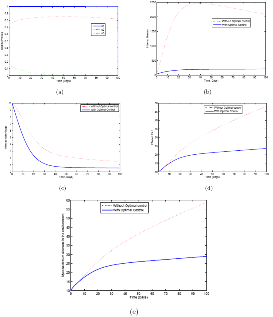Figure 5.4. Shows the profile of the optimal control u1,u2,u3 and optimal solution for infected humans, water bugs, small fish and MU in environment via mass treatment, insecticide application and mass education

6. Conclusions

In this study, we derived and analyzed a deterministic model for the spread of Buruli ulcer that includes mass treatment, insecticide and mass education. We determine the basic reproduction ratio . This ratio depicts the existence and the stability of the equilibra of the model. Applying optimal control strategy, we find a solution to the eradication of BU disease in a finite time. By observing the numerical results, we can conclude that the combination of all the control , and are capable of helping reduce the number of infected humans, water bugs, small fishes and MU in the environment.