Jean Roger Bogning
Department of Physics, Higher Teachers Training College, University of Bamenda, PO Box 39, Bamenda, Cameroon
Correspondence to: Jean Roger Bogning , Department of Physics, Higher Teachers Training College, University of Bamenda, PO Box 39, Bamenda, Cameroon.
| Email: |  |
Copyright © 2014 Scientific & Academic Publishing. All Rights Reserved.
Abstract
The dynamics of propagation of waves in the transmission supports as high-nonlinear and dispersive optical fibers is governed by Schrödinger equations that integrate supplementary nonlinear terms. This particularity complicates the resolution of this equation. So the resolution of such an equation requires a suitable method. In this article, we construct solutions of the type solitary wave by means of a method which supposes from the onset that the equation admits a solution that is a combination of the bright soliton and dark soliton and thereafter proceed by elimination of the constants until the exact solutions or those that are nearer to the exact solutions are obtained.
Keywords:
Solitary wave, Schrödinger equation, Optical fibers, Bright soliton, Dark soliton
Cite this paper: Jean Roger Bogning , Solitary Wave Solutions of the High-order Nonlinear Schrödinger Equation in Dispersive Single Mode Optical Fibers, American Journal of Computational and Applied Mathematics , Vol. 4 No. 2, 2014, pp. 45-50. doi: 10.5923/j.ajcam.20140402.02.
1. Introduction
The nonlinear partial differential equations that describe the propagation of waves in the atomic chains, electric lines and optical fibers are for most of schrödinger’s type. They present nonlinear terms that are most often of cubic order, quintic and so on. The research of the analytical solutions for these equations is never an easy task. It is justified besides by the multitude of mathematical methods that many authors use every day in the resolution of mathematical problems [1-13]. The nonlinear partial differential equations that describe the propagation of waves in the atomic chains, electric lines and optical fibers are for most of schrödinger’s type. If we come back to the optical fiber transmission support that is currently in the center of modern telecommunications, one realizes that in the case of high-nonlinear dispersive single mode optical fiber, the dynamics of propagation of waves is governed by the following Schrödinger equation [14].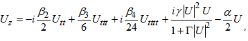 | (1) |
where  is the slowly varying amplitude of the electrical field envelope,
  is the
  order of the dispersion parameter,
  is the linear loss parameter,
  is the parameter of saturation of the nonlinearity and
  designates the magnitude of the kerr parameter and nonlinear absorption and
 . This nonlinear partial differential equation is not easy to solve. This difficulty to solve is translated by very few works that propose analytical solutions of this equation as presented above. Our aim in this work is to propose some analytical solutions to this equation, or merely to find the solutions very close to the exact solutions. The equation (1) is high-nonlinear and dispersive; then susceptible to have some solitary solutions. Thus, the method of research of the solutions, consist in supposing initially that the equation (1) admits a solution that is a combination of solitary waves of nature bright and kink of the shape
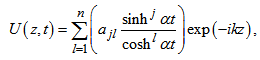 | (2) |
where  ;
;  ;
; ;
;  designates the number of terms of equation (2);
  ,
,  and
and  the constants to determine as a function of the parameter of the equation (1). When the equation (2) and its different derivatives are introduced in the equation (1), we get the complicated coefficient equations and of which the elimination of the constants case by case, permits to obtain the solutions progressively. In this work, we will limit in the case where we have four complex coefficients
 . So the manuscript is presented as follows: In section 2, we obtain the equations of the coefficients
 . In the section 3, we analyze the different possibilities of obtaining the solutions. Finally section 4 concludes our work.
2. Coefficient Equations
After reducing in the same denominator, equation (1) becomes | (3) |
The aim is to construct explicitly the solutions of equation (2) in the form | (4) |
where the coefficients  of equation (2) are substituted by
  ,
,  ,
,  and
and  are complex numbers such that
  ,
,  ,
,  ,
,  ,
,  ,
,  ,
,  and
and  are real constants to be determined as a function of the parameters of the system. So equation (3) inserted into equation (1) yields
 | (5) |
where  ,
,  ,
,  ,
,  and
and  are function of the constants
  ,
,  ,
,  ,
,  ,
,  ,
,  ,
,  and
and  . From the real and imaginary part of equation (5), we obtain according to the terms in
  and
and  the series of equations
 | (6) |
and | (7) |
Similarly the terms in  and
and  lead to the following equations
 | (8) |
and | (9) |
Equations (4), …, (7) are the main equations which permits to investigate the form of solutions as in equation(4). Since these equations have eight unknowns, and not easy to solve, we proceed by different analyses.
3. Analysis of the Solutions
a) First case:  ,
,  ,
,  ,
,  From equations (6) and (7) we obtainTerm in
  ,
, | (10) |
Term in  ,
, | (11) |
Term in  ,
, | (12) |
Term in  ,
, | (13) |
The combination of equation (10) and (11) gives | (14) |
Insertion of (14) in (12) and (13) respectively yields | (15) |
and | (16) |
where  ;
;  ,
,  ,
,  ;
;  ,
,  . Eliminating between equation (13) and (14) gives the quadratic equation
 | (17) |
where the coefficients  ,
,  and
and  are given by
  ;
;  and
and  . - For
  , i.e.
  we obtain
 | (18) |
 | (19) |
 | (20) |
The resulting solution of equation (3) in this case is given by | (21) |
− For  ; i.e.
  , we obtain when
  the following values
 | (22) |
 | (23) |
and | (24) |
The resulting solution of equation (3) in this case is given by | (25) |
− For  , equation (25) reads
 | (26) |
b) Second case: only  ;
;  We obtain from order
  to
to  of equation (6) and (7), the following equations
 | (27) |
and | (28) |
From equations (27) and (28) one finds | (29) |
and | (30) |
Here, the solution of equation (3) is given by | (31) |
c) third case: only  ,
,  From the terms in
  and
and  of equations (6) and (7) the equations
 | (32) |
and | (33) |
Substituting equation (33) into equation (32) with the constraint  gives the solution of the form
 | (34) |
d) Fourth case: only  and
and  We obtain for any parameter coefficient of the nonlinear partial differential equation (3)
  . So the solution of equation (3) in this case is given by
 | (35) |
e) Fifth case: only  ,
,  From the order
  to order
  of equations (6) and (7), we obtain
  and the solution is given by
 | (36) |
f) sixth case: only  ,
,  Here both right-hand side and left-hand side of the obtained equations (6),…, (9) vanish for
  . Then any solution of the following form verify equation (3)
 | (37) |
where  and
and  are real numbers.g) Seventh case: only
  The equation which derives from the term in
  gives
gives  with
with  . The solution in this case is given by
 | (38) |
4. Conclusions
To start the research of solutions as proposed in this manuscript, we remark that in numerous studies of the modulational instability proposed by most authors on the equation (1), the perturbated solution is most often a plane wave and very rarely a solitary wave. This is how we took the option to determine some solitary waves of this equation. Knowing that there is no standard method of resolution of the nonlinear partial differential equations, we have use the effective method as used in this manuscript to attain our objective. Certainly it necessitates a lot of concentration, but also gives a lot of satisfaction. Apart from the above solutions obtained, the following cases: ;
;  ;
;  ;
;  ;
; lead to trivial solutions or impossibilities. This principle of looking for solution maybe extended to other types of nonlinear partial differential equations susceptible to have some solitary wave solutions. A numerical approach can also be considered.
References
| [1] | R. Hirota, The Method in soliton theory, Cambridge University press, 2004. |
| [2] | W. Hereman and A. Nuseir, Symbolic methods to construct exact solutions of nonlinear partial differential equations, Mathematics and Computers in Simulation, Vol. 43, pp. 13-27, 1997. |
| [3] | M. J. Ablowitz, P. A. Clarkson, Solitons, Nonlinear evolution equations and inverse scattering, Cambridge University press, London, 1991. |
| [4] | V. B. Matveev, M. A. Salle, Darboux transformation and solitons, Springer_Verlag, Berlin, 1991. |
| [5] | A. M. Wazwaz, A new fifth order nonlinear integrable equation: multiple soliton solutions, Physica Scripta, Vol. 83, pp. 015012-015016, 2011. |
| [6] | A. M. Wazwaz, The Hirota’s direct method and the tanh-coth method for multiple soliton solutions of the Sawada- Kotera-Ito seventh-order equation, Applied Mathematics and Compution, Vol. 199, pp. 133-138, 2008. |
| [7] | J. R. Bogning, C. T. Djeumen Tchaho, T. C. Kofané, Construction of the soliton solutions of the Ginzburg-Landau equations by the new Bogning-Djeumen Tchaho-Kofané method, Physica Scripta, Vol. 85, pp. 025013-025018, 2012. |
| [8] | J. R. Bogning, C. T. Djeumen Tchaho, T. C. Kofané, Generalization of the Bogning-Djeumen Tchaho-Kofané method for the construction of the solitary waves and the survey of the instabilities, Far East Journal of Dynamical systems, Vol. 20, No. 2, pp.101-119, 2012. |
| [9] | C.T. Djeumen Tchaho, J. R. Bogning, T. C. Kofané, Modulated Soliton solution of the Modified Kuramoto- Sivashinsky’s equation, American Journal of Computational and Applied Mathematics, Vol. 2, No. 5, pp. 218- 224, 2012. |
| [10] | C. T. Djeumen Tchaho, J. R. Bogning, T. C. Kofane, Multi-Soliton solutions of the modified Kuramoto- Sivashinsky’s equation by the BDK method, Far East Journal of dynamical systems, Vol.15, No.2, pp. 83-98, 2011. |
| [11] | J. R. Bogning, T. C. Kofane, Analytical Solutions of discrete nonlinear Schrödinger equation in arrays of optical fibers, Chaos, Solitons &Fractals, Vol. 28, pp. 48-153, 2006. |
| [12] | J. R. Bogning, Pulse soliton Solutions of the modified KdV and Born- Infeld Equations, International Journal of Modern Nonlinear Theory and Applications, Vol. 2, pp. 135-140, 2013. |
| [13] | J. R. Bogning, C. T. Djeumen Tchaho, T. C. Kofané, Solitary wave solutions of the modified Sasa- Satsuma nonlinear partial differential equation, American Journal of Computational and Applied Mathematics, Vol. 3, No. 2, pp. 97-107, 2013. |
| [14] | M. N. Zambo Abou’ou, P. Tchofo Dinda, C. M. Ngabireng, B. Kibler, F. Smektala, K. Porsezian, Suppression of the frequency drift of modulational instability sidebands by means of fiber system associated with a photon reservoir Optics Letters, Vol. 36, No 2, pp. 256-258, 2011. |
 Abstract
 Reference
 Full-Text PDF
 Full-text HTML