Sudipa Chauhan 1, Om Prakash Misra 2, Joydip Dhar 3
1Amity Institute of Applied Sciences, Amity University, Noida, India (Amity University)
2School of Mathematics and Allied Sciences, Jiwaji University, Gwalior, M.P, India
3ABV-IIITM, Gwalior, India (ABV-IIITM, Gwalior)
Correspondence to: Sudipa Chauhan , Amity Institute of Applied Sciences, Amity University, Noida, India (Amity University).
| Email: |  |
Copyright © 2012 Scientific & Academic Publishing. All Rights Reserved.
Abstract
This paper aims to study a SIR model with and without vaccination. A reproduction number R0 is defined and it is obtained that the disease-free equilibrium point is unstable if  and the non-trivial endemic equilibrium point exist if
  in the absence of vaccination. Further, a new reproduction number
  is defined for the model in which vaccination is introduced. The linear stability and the global stability of both the models are discussed and the comparison of both the models is done regarding the existence of the disease-free equilibrium point and endemic equilibrium point. Finally, a numerical example is given in support of the result.
Keywords:
SIR model, Reproduction number, Stability, Vaccination
Cite this paper: Sudipa Chauhan , Om Prakash Misra , Joydip Dhar , Stability Analysis of SIR Model with Vaccination, American Journal of Computational and Applied Mathematics , Vol. 4 No. 1, 2014, pp. 17-23. doi: 10.5923/j.ajcam.20140401.03.
1. Introduction
Diseases are the main threat in today’s society. Urbanization and other factors which are making our life easier to live on the other hand are major cause of diseases. These diseases then lead to huge epidemic and the result is big loss of population. Hence, the modeling of infectious diseases is very important so that it can be controlled and the epidemic can be reduced. It is a tool which is used to study the mechanism by which the strategies can be made to control the epidemic.An epidemic model is a simplified means of describing the transmission of communicable disease through individuals. Since many years, the outbreak of disease has been questioned and studied. The ability to make predictions about diseases is expected to enable scientists in evaluating inoculation or isolation plans which will further have significant effect on the mortality rate of particular epidemic. The SIR model in epidemiology gives a simple dynamic description of three interacting populations, the Susceptible, the Infected, and the Recovered. In spite of its simplicity, the SIR model, exhibits the basic structure generally associated to the spread of a disease in a population: after a possible initial epidemic, the infected population either tapers to zero or to a stable endemic level. Many variations of the SIR model have been studied in recent years to more accurately model more complex diseases and infection mechanisms. For instance the susceptible population may be divided into subgroups with different infection rates[1,4,5,6,11], the disease may affect reproductive rates in the infected or recovered population[2], or there may be multiple levels of infections, some lethal, some sublethal[3, 7]. These more complicated models can lead to instabilities, and even cyclic behavior in the infected population. There are many diseases that bring great economic and human cost to society which accommodate multiple infection routes. Other than through direct contact, diseases are often transmitted through animal or insect vectors (e.g. malaria or plague), through fecal contamination of water or food supplies (cholera, typhus, avian influenza), or through ingestion of infected tissues (brucellosis, bovine spongiform encephalopathy). Detailed modeling of these infection routes can be quite complicated, involving such issues as the life cycle of the vector, or the diffusion of infected materials through water sources. The model we study does not attempt to understand the details of such mechanisms, but, as with the SIR model, is meant as a broad conceptual tool for giving rudimentary insight into the general behavior of the dynamics of such diseases.In this paper, we discuss the stability analysis of susceptible-infected-recovery (SIR) epidemic model with and without vaccination. The disease-free equilibrium point, endemic equilibrium point of the model is discussed. The local and global stability analysis of the model is determined by the basic reproduction number. Models with a similar feedback mechanism were studied in[8, 9, 10].The paper is organized as follows: In section 2, we have presented our model 1, description of parameters, linear stability, global stability of disease free and endemic equilibrium point. In section 3, we have presented our Model 2 and its stability analysis. In section 4, we have given a numerical example in support of our result and in the last section conclusion is given followed by the application of the models. SIR model is studied earlier by many researchers but we have extended it by the linear, global stability analysis and a numerical example in support of our result. Further we have compared the result with Model 2 in which we have included vaccination. The results are also supported by the graphs in the section of numerical example.
2. Mathematical Model & Stability Analysis (Model 1)
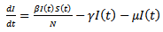
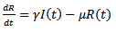
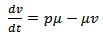
The SIR Model is used in epidemiology to compute the amount of susceptible, infected, recovered people in a population. This model is an appropriate one to use under the following assumptions:• The population is fixed.• The only way a person can leave the susceptible group is to become infected. The only way a person can leave the infected group is to recover from the disease. Once a person has recovered, the person received immunity.• Age, sex, social status, and race do not affect the probability of being infected.• There is no inherited immunity.• The member of the population mix homogeneously (have the same interactions with one another to the same degree).• The natural birth and death rates are included.• All births are into the susceptible class.• The death rate is equal for members of all three classes, and it is assumed that the birth and death rates are equal so that the total population is stationary.As defined earlier:The model starts with some basic notation:• S (t) is the number of susceptible individuals at time t.• I (t) is the number of infected individuals at time t• R (t) is the number of recovered individuals at time t• N is the total population sizeThe assumptions lead us to a set of differential equations: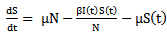 | (1) |
 | (2) |
 | (3) |
where S (t) is the number of susceptible at time t, I (t) is the number of infected people at time t, R (t) is the number of recovered at time t, β is the transmission of disease from an infected person in a time period, μ is the is the death and birth rate which are assumed to be equal, γ is the recovery rate and the population size is constant, so that N = S (t)+I (t)+R (t)And 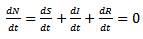 | (4) |
For simplicity, we can consider the prevalence i.e. the proportions by redefining  Substituting the above assumptions in equations (1), (2) and (3), we get
 | (5) |
Similarly we get, | (6) |
 | (7) |
with the initial conditions Here μ is the recruitment and natural death rate,
  is the effective contact rate between susceptible and infected individuals and
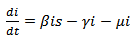
  is the recovery rate of infected individuals.By considering the total population density, we have
  Therefore it is enough to consider
 | (8) |
 | (9) |
The following set is positively invariant for the above system of equations: There are two equilibrium points that exists for above model:1. Disease-free Equilibrium Point
  2. Endemic equilibrium point
 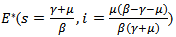 REMARK 1: The endemic equilibrium point exists only when
  i.e the infection rate must be greater than the death rate of the infected individuals or
 , where
  is known as reproduction number which determines the asymptotic behavior of the model. Reproduction number is the number of secondary infection occurring from the primary infection.Further, in order to obtain the positive equilibrium points of the system, we solve i from the equation (8) and obtain
 we substitute this into the second equation, which yields to
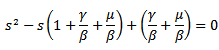 The discriminant of the above equation is
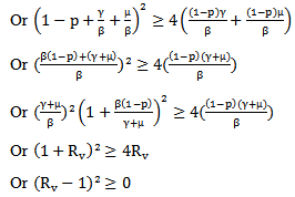
 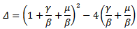 Then for the positive solution of the equation
  Or
Or 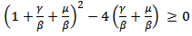 0r
0r  which is again equivalent to
  Now we will be studying the linear stability of both the equilibrium points by Jacobian.
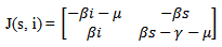 The jacobian matrix evaluated at
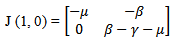 The characteristic equation corresponding to the disease free equilibrium point is
  which gives the eigenvalues
  and
and  .Here,
  . Now, considering
 ,If β – μ – γ < 0 then
  or
or  or
or  Then, the disease-free equilibrium point is locally asymptotically stable as both the eigenvalues are negative. For any infectious disease, one of the most important concerns is its ability to invade a population. This can be expressed by a threshold parameter
 . The infected individual in its entire period of infectivity will produce less than one infected individual on average if
 . In disease-free equilibrium point case, the system is locally asymptotically stable. This shows that the disease will be wiped out of the population. Moreover infected group exists only if
  The disease-free equilibrium point is unstable if β – μ – γ > 0 or
  because if
 , then the each infected individual in its entire infective period having contact with susceptible individual will produce more than one infected individual, which will then lead to the disease invading the susceptible population, and the disease-free equilibrium point will become unstable.
 Note that coefficients
  and
and  are both positive.The roots of the above polynomial or the eigenvalues are:
 Or
Or Since μ(β-γ-μ) is positive, the quantity under the square root is either smaller than
 , or greater than
 . If
. If  than the eigenvalues are complex with the real part
 , which is negative. If
  then the quantity under the square root must be smaller in absolute value than
 , but still the real part is negative. Either way, we conclude that the endemic equilibrium is stable since the real parts of both eigenvalues are negative. It shows that the endemic equilibrium point is stable i.e. both the susceptible and infected population will survive in either of the cases and the trajectories will approach to the endemic equilibrium point.REMARK 2: It is concluded from the linear stability of the equilibrium points that the disease-free and endemic equilibrium point cannot exist simultaneously. If
 , then the disease-free equilibrium point is stable and if
 , then the endemic equilibrium point is stable.THEOREM 1 If
 , then the disease free equilibrium point of the system is globally asymptotically stable on
  .PROOF To establish the global stability of the disease free equilibrium point, we construct the following Lyapunov function
 Then, the time derivative of V is
 Thus
Thus  for
for  Further
  if i(t)=0 or s(t)=1 and
  Hence, the largest invariant set contained in the set
  is reduced to disease free equilibrium point. Since we are in compact invariant set, hence by Lasalle invariance principle, the disease-free equilibrium point is globally asymptotically stable in
  [15].REMARK 3: Unlike Lyapunov’s theorems, LaSalle’s principle does not require the function V(x) to be positive definite. If the largest invariant set M, contained in the set E of points where
  vanishes, is reduced to the equilibrium point, i.e. if
  , the LaSalle’s principle allows to conlude that the equilibrium is attractive. But a drawback of Lasalle’s principle, when significant, is that it proves only the attractivity of the equilibrium point. It is well known that in the nonlinear case attractivity does not imply stability. But when the function V is not positive definite, Lyapunov stability must be proven. This is why LaSalle’s principle is often misquoted. Some additional condition enables, with LaSalle’s principle, to ascertain asymptotic stability. To obtain stability from LaSalle’s principle some additional work is needed. The most complete results, in the direction of Lasalle’s principle to prove asymptotic stability, have been obtained by LaSalle himself (LaSalle:[13], in 1968, completed in 1976 [14].)THEOREM 2 The endemic equilibrium point
  of the system is globally asymptotically stable on
  .PROOF: We construct a Lyapunov function
  where
where  given by
  Where
Where  are positive constants to be chosen later. Then the time derivative of the Lyapunov function is given by
 considering the equilibrium point we get,
  and
and  . Thus, we get the following equation
 For W1 =W2=1,
  Also, if s=s* then
 Hence, by Lasalle invariance principle, the endemic equilibrium point is globally asymptotically stable.
3. Mathematical Model & Stability Analysis (Model 2)
Now, we present our second model in which we have also induced vaccination and the suggested model is as follows: 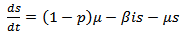 | (10) |
 | (11) |
 | (12) |
 | (13) |
where s are the susceptible, i are infected population, r is the recovered population and v is the group to which vaccination is given, μ is the mortality rate, p is the vaccination rate, γ is the recovery rate and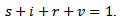 By considering the total population density, we have
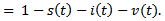 Therefore it is enough to consider
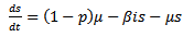 | (14) |
 | (15) |
 | (16) |
The feasible region for the above system is There are two equilibrium points that exists for above model:1. Disease-free Equilibrium Point E0(s=1-p , i=0, v=p)2. Endemic equilibrium point
  In order to show the existence of endemic equilibrium point, we calculate the value of i from (14) and is substitute it in equation (15), which yields to
 The discriminant of the above equation is
  Then for the positive solution of the equation
 Which is equivalent to
  REMARK 4: The effect of vaccination can be easily seen on the existence of the disease-free equilibrium point and endemic equilibrium point. The susceptible population has decreased by a parameter p (vaccination rate). Further a major impact is on the reproduction number i.e. the number of secondary infections. The new reproduction number is
  after the induction of vaccination in the model. The endemic equilibrium point will only exist if
 .Now we will be studying the linear stability of the disease- free equilibrium point and the endemic equilibrium point.The characteristic equation corresponding to the disease -free equilibrium points is
 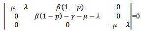 The above determinant gives three eigenvalues:
 Here,
Here,  and
and  are negative. Now considering
  ,• If
,• If  which means
  Hence,
  or
or  which means that the disease -free equilibrium point is not locally asymptotically stable.• If
  which means
  Hence,
  or
or  which means that the model is linearly stable as all the eigen values are negative and hence there is no epidemic and the trajectories will approach to disease-free equilibrium point.
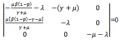 Solving the above determinant we get:
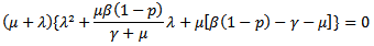 Note that coefficients
  and
and  are both positive.On solving the above equation we get the following eigen values:
 Or
Or Since
Since  is positive, the quantity under the square root is either smaller than
  , or it is greater. If greater, then the solutions are complex with real part
 which is negative. Otherwise, the square root must be smaller in absolute value than
  , but still the real part of the eigenvalue is negative. Either way, we conclude that the endemic equilibrium is stable since the real parts of both eigenvalues are negative and
  is also negative. It shows that the endemic equilibrium point is locally stable i.e. both the susceptible and infected population will survive in either of the cases and it can be seen that the infection rate has reduced because of the vaccination parameter i.e. p.Now, we jump to the global stability of the disease free equilibrium point and the endemic equilibrium point.THEOREM 3 The disease-free equilibrium point of the system is globally asymptotically stable on
  .PROOF To establish the global stability of the disease free equilibrium point, we construct the following Lyapunov function
 Then, the time derivative of V is

 Thus, if
  then
then  and the disease -free equilibrium point is globally asymptotically stable. Further, at
  ,
,  . Hence, by LaSalle’s invariance principle, the disease-free equilibrium point is globally asymptotically stable.THEOREM 4 The endemic equilibrium point
  of the system is globally asymptotically stable on
  .PROOF: We construct a Lyapunov function
  where
where 
 given by
 where
where  are positive constants to be chosen later. Then the time derivative of the Lyapunov function is given by
 Considering the equilibrium points, we get
 and
and  and putting the values in the above equation we obtain
 If
If  then
then  and if
  and
and  then
then  . Hence, by LaSalle invariance principle, the endemic equilibrium point is globally asymptotically stable.
4. Numerical Examples
We will discuss the results of both the models by taking a numerical example. We consider the parameters μ =0.5, β= 1.98time-1, γ=0.5 for the model 1 without vaccination and conclude that the susceptible population decreases to a lower level due to the effect of infection rate β (Figure 1). The endemic equilibrium point is (0.5052, 0.2470).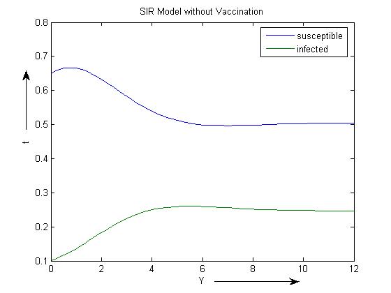 | Figure 1. SIR model without vaccination with β =1.98 |
Gradually, we increased the infection rate β =2 and saw that the susceptible population declines to a lower level. The endemic equilibrium point is (0.5002, 0.2495). (Figure 2)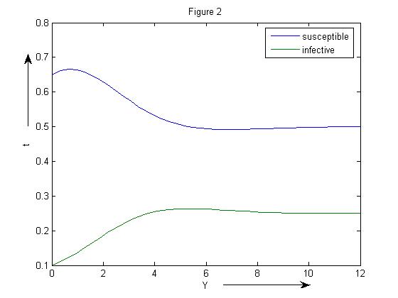 | Figure 2. SIR model without vaccination with β=2 |
The endemic equilibrium point corresponding to β=2.5 is (0.4002, 0.2999) (Figure 3).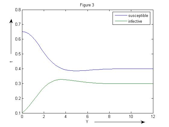 | Figure 3. SIR model without vaccination with β=2.5 |
The endemic equilibrium point for β=3.5is (0.2857, 0.3572) (Figure 4)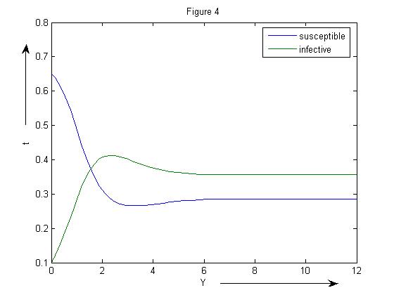 | Figure 4. SIR model without vaccination with β =3.5 |
REMARK 5: It can be easily seen that the susceptible population declines to half of its level due to the presence of infection and the infected population suddenly rises because of infection. As the infection rate increases, the susceptible population decreases and the infected population gradually increases and at β =3.5, the infected population becomes more as compared to the susceptible population.Further, the linear stability of both the points are calculated and it is concluded that the eigen values of the disease free equilibrium point is 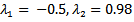 and the reproduction number is 1.98>0. Thus it confirms our result that when
 , the trajectories cannot approach towards the disease free equilibrium point. The characteristic equation of the endemic equilibrium point is given by
 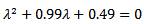 and the eigen values are
 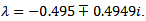 Since the real parts of both the eigenvalues are negative, hence the endemic equilibrium is stable which again confirms our theoretical result that at
  , the endemic equilibrium point is linearly stable.Now, we have taken the same set of parameters and also added the parameter p=0.6 as a vaccination rate for model 2 i.e with vaccination. The endemic equilibrium point corresponding to model 2 is (0.3858, 0.0050, 0.3995). Figure 5).
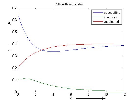 | Figure 5. SIR model with vaccination with β =3.5 |
REMARK 6: The susceptible population decreases to a lower level due to vaccination. Further, the infected population declines drastically due to vaccination and the vaccinated population increase which can be seen from the above graph.The reproduction number 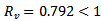 concludes that the disease free equilibrium point is stable. The eigenvalues corresponding to the disease free equilibrium point are
 Hence, it is linearly stable. Thus, we can see that when we apply vaccination in the SIR model, the infected population which was at 0.2470 decreases to 0.0050 at the infection rate β =1.98 due to the effect of vaccination.
5. Conclusions
In this paper, two models have been discussed. In the models, the effects of disease on populations with and without vaccination are discussed. For both the models it is found that the dynamics of the infection were dependent on the value for the basic reproductive ratio i.e. Rv or R0. In model 1, it is observed that disease-free equilibrium state (DFE), exist only when the reproduction number  is less than 1 and all the trajectories will be approaching towards the DFE. The linear and global stability of the disease free equilibrium point is also discussed. Further, it is noticed that both the equilibriums, disease free equilibrium and endemic equilibrium cannot exist together. The endemic equilibrium can only exist when
  is greater than 1. The linear and global stability of the endemic equilibrium point is also discussed.In comparison to model 1, in model 2 where the vaccination is induced, a drastic change in the reproduction number is observed and it changed from
  to
to
 . Again, the disease-free equilibrium point is stable when
  and the trajectories approach to endemic equilibrium point when
  . Further, the effect of infection rate is also seen on the susceptible and infected population. The susceptible population gradually decreases and infected population increases as the infection rate β increases. But as we induce vaccination in the susceptible population, the infected population suddenly decreases to a very lower level. Thus, we can conclude that the infection rate and reproduction number plays a very important role for an epidemic to occur and this epidemic can be controlled by vaccination.
6. Application
The above two models are very useful for controlling the epidemics in a given population in a particular region or locality. There are number of diseases like influenza, HINI, dengue and many more in developing countries like India, Indonesia etc. According to the models which we have studied, the feasibility of controlling an epidemic critically depends on the value of  and
and . The more severe the epidemic (i.e. the greater the value of
  or
or ) the more intensive the intervations must be to significantly reduce the number of infections and deaths. Not surprisingly, the levels of vaccination or treatment necessary for control are lower if interventions are targeted. For e.g.[11,12] modeled the effects of age-specific targeting strategies and found vaccinating 80% of children (less than 19 years old) would be almost as effective as vaccinating 80% of the entire population. In the next paper, we will be extending our model by including the parameter of targeted individuals to be vaccinated, so that we can see the effect of it on the reproduction number.
ACKNOWLEDGEMENTS
I am very much thankful to my guides Dr. Om Prakash Misra and Dr. Joydip dhar for their constant and continuous guidance whenever required.
References
| [1] | R.M.Anderson, R.M. May,”Infectious Diseases of Humans”, Oxford UniversityPress,Oxford, 1991. |
| [2] | R.M.Anderson, R. M., May,” The Population Dynamics of Microparasites and their Invertibrate Hosts” Philosophical Transactions of the Royal Society of London, Series B, Biological Sciences, 291, 451-524,1981. |
| [3] | M.Boots, R. Norman,” Sublethal infection and the population dynamics of host-microparasite interactions”, J. Animal Ecology, 69, 517-524,2000. |
| [4] | L. Esteva, C. Vargas,” Analysis of a dengue disease transmission model”, Math. Biosciences, 150,131-151,1998. |
| [5] | G.MacDonald,” The Epidemiology and Control of Malaria”, Oxford University Press, London, 1957. |
| [6] | Obara, “Mathematical Models in Epidemiology”, Master’s Thesis University of Georgia, 2005. |
| [7] | S.M.Sait, M.Begon, D.J. Thompson.,” The effects of a sublethal baculovirus infection in the Indian meal moth, Plodia interpunctella.” J. Animal Ecology, 63 ,541-550,1994. |
| [8] | H.R.Thieme,”Pathogen competition and coexistence and the evolution of virulence”, Mathematics for Life Sciences and Medicine. (Y. Takeuchi, Y. Iwasa, K. Sato, eds.), 123-153, Springer, Berlin Heidelberg 2007. |
| [9] | M.Zhien, J.Liu, J. Li ,” Stability analysis for differential infectivity epidemic models”, Nonlinear Analysis: Real World Applications, 4, 841-856,2003. |
| [10] | M.A.Nowak, A.R.Mclean,” A mathematical model of vaccination against HIV to prevent the development of AIDS, Vol.246, No.1316, Nov.22,1991. |
| [11] | J.Arino, C.Mccluskey, P.V.Driessche, “Global results for an epidemic model with vaccination that exhibits backword bifurcation”, Siam Journal of Applied Mathematics, Vol. 64, No.1, pp.260-276,2003. |
| [12] | Longini.et.al, ”Strategy for distribution of Influenza Vaccine to High-Risk Groups and Children”, American Journal of Epidemiology,161(4),303-306,2005. |
| [13] | P. LaSalle, Stability theory for ordinary differential equations, J. Differ.Equations, 41:57–65, 1968 |
| [14] | J.P. LaSalle, Stability of non autonomous systems, Nonlinear Anal., Theory, Methods Appl., 1(1):83–91, 1976. |
| [15] | P. LaSalle and S. Lefschetz, Stability by Liapunov’s direct method, Academic Press, 1961. |
 Abstract
 Reference
 Full-Text PDF
 Full-text HTML