Ali Filiz
Department of Mathematics, Adnan Menderes University, Aydin, 09010, Turkey
Correspondence to: Ali Filiz, Department of Mathematics, Adnan Menderes University, Aydin, 09010, Turkey.
| Email: |  |
Copyright © 2012 Scientific & Academic Publishing. All Rights Reserved.
Abstract
In this study, we investigate convergence properties of time and space discretization of Parabolic Volterra integro-differential equations (PVIDE) is outlined. The rectangle and the trapezoidal rules applied for integral term of these equations and finite difference method (Backward-Euler method) used for partial differential part. The integral is approximated in each case by the quadrature rule with relatively high-order truncation error. We consider time step methods based on the backward-Euler method and combined with the appropriate quadrature rules.
Keywords:
Finite difference method, Backward-Euler method, Parabolic volterra integro-differential equations, Integral equations, Partial differential equations, Time and space discretization, Mixed rule, Quadrature rule, Error
Cite this paper: Ali Filiz, Numerical Solution of Parabolic Volterra Integro-Differential Equations via Backward-Euler Scheme, American Journal of Computational and Applied Mathematics , Vol. 3 No. 6, 2013, pp. 277-282. doi: 10.5923/j.ajcam.20130306.02.
1. Introduction
In[5] and[1], Linz and Baker considered the numerical solution of Volterra integral equations of the second kind using the rectangle, the trapezium and Simpson’s rules for finding  with the quadrature rule. Whereas, in this paper we introduce the numerical treatment of parabolic Volterra integro-differential equations using the backward-Euler scheme for finding
  with the finite difference method. In[2], Douglas introduced the numerical treatment of parabolic Volterra equations using the backward-Euler and Crank-Nicolson methods for finding
  with the finite difference method of the form
 | (1) |
Douglas’s has used quite simple equation, but it is important that he used firstly time discretization using the backward-Euler and Crank-Nicolson methods. However, In[2] and[7] the numerical examples are not given. In this paper the time and space discretization are studied with examples. In this paper we will study the numerical solution by the time-continuous finite difference method of parabolic Volterra equations of the form  | (2) |
in  In the
  plane let

 and let
  have the initial and boundary conditions
  on
on 
 =0.Here we denote by
  the closure of
  is an elliptic second order partial differential operator and
  is a second order partial differential operator respectively.We assume that both operators are smooth. The equation (2) is to be solved subject to the above initial and boundary conditions. As they defined in[5] and[1], the kernel
  is a smooth, real-valued function of both variables for
  and
and  is supposed to be a smooth function of
  The numerical methods will be a combination of finite difference and quadrature schemes for the time stepping, with time step
  . Introducing a lattice in
  we define for positive integers
  and
and 


 For any function
  defined on
  we set
  We replace the time derivative in (2) by a difference quotient, and use a quadrature rule for the integral term of the form
 | (3) |
where  a quadrature is weight and
  is the approximation to
2. Numerical Methods for Parabolic Volterra Integro-differential Equations
In this section we will study the initial boundary value problem first considered in the introduction, i.e., | (4) |
in  In the
  plane let

 and let
  have the initial and boundary conditions
  on
on 
 =0.One of the difficulties involved in such a method is that if
  for j ≤ n, then all values of
  have to be retained, causing great demands for data storage. In Sloan and Thomée[7] a quadrature rule based on fewer points is proposed, thus reducing the number of time levels at which the data need be saved.The quadrature rule will be of the form
 | (5) |
We define the backward difference method by | (6) |
The simplest quadrature rule of type (3) which is consistent with the order of accuracy of the backward-Euler scheme is the rectangle rule | (7) |
which corresponds to choosing  for 0 ≤ j ≤ n − 1, so that
 | (8) |
Let  and
and  Set
Set  and let
  be the largest integer such that
  In approximating the integral term over
  we shall apply the trapezoidal rule with step size
  on
on  and the rectangle rule with step-size
  on the remaining part
  . More precisely, with
 | (9) |
Note that this rule has a storage requirement of  as opposed to
  for the simple rectangle rule. Sloan and Thomée[7] deal with stability and convergence results for two different time discretization of (6), based on the backward-Euler and Crank-Nicolson methods respectively. In their paper, the time discretization is studied in the treatment of the integral term. Let k be the time step in the backward-Euler scheme for the equation
 | (10) |
or for the following form with elliptic operator under the integral term, | (11) |
If we substitute the backward difference for  centred difference for
  in (10), and a quadrature rule for the integral term, we obtain the following form
 | (12) |
and if we substitute the backward difference for  centred difference for
  in (11), and a quadrature rule for the integral term, we obtain the following form
 | (13) |
where h is the mesh step for x. The sum on the RHS is the quadrature approximation to the integral term of (10) or (11) at the point  The weights in the quadrature rule correspond to (9) above. For sufficiently regular functions g the truncation error is of order
  assuming that t is bounded. If we take
  the accuracy is similar to that of the backward-Euler scheme. If the weights
  are trapezoidal weights for step-size
  and
and  are rectangle rule weights for step-size k, we can write
 | (14) |
From (14) we have | (15) |
where, as easily verified (assuming  ),
), | (16) |
Note that in the numerical solution of Example 2.1, Example 2.2 and Example 2.4, we did not include the function  Examples with the function
  can be done in a similar manner. Example 2.1: Consider the initial-boundary value problem
 | (17) |
for 
 with
with 
 and
and  which has the exact solution
 | (18) |
where  and
and  .Taking
  = 1 in the equation (18) we have the solution
 | (19) |
If we put  in (18) we obtain the solution
 | (20) |
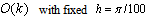
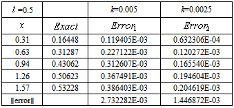
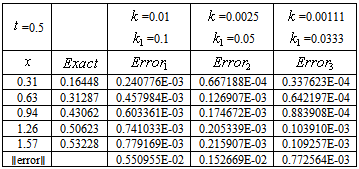
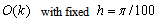
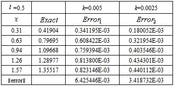
The last result corresponds to the simplest form of our main problem (17). We will solve the equation (17) with the backward-Euler method. Firstly, we use the rectangle rule throughout for the integral term in equation (17). Table 1 shows numerical results for this case. Unless otherwise indicated, throughout this section and the next section we take  and T = 0.5. Table 1 shows that the combined backward-Euler and rectangle rule has error O(k) for this Example 2.1
Table 1. Rectangle rule showing effect of time-step k, for Example 2.1, has an error of order
 |
| |
|
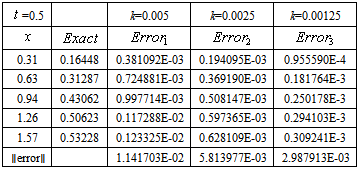
In this test we see that the space error has the expected order in our numerical calculations. Secondly, we use the trapezoidal rule throughout for the integral term in equation (17). The numerical results are given by Table 2. Thirdly, we obtain the numerical solution of equation (11) using the trapezoidal rule and rectangle rule as in (9) which is called the mixed rule. Table 2 illustrates that the combined backward-Euler and trapezoidal rule also has error of order k for Example 2.1Table 2. Trapezoidal rule showing effect of time-step k, for Example 2.1, has an error of order
 |
| |
|
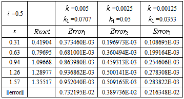
Table 3 shows numerical results for the mixed rule (backward-Euler scheme). In Table 3, we take m = integral part of  for the cases in Table 3, we have
  = integer. First, we will apply the simplest rule which is the rectangle rule for the integral term. Table 3 illustrates that the combined trapezoidal and rectangle rule has error of order k for Example 2.1.
Table 3. Mixed rule showing effect of time-step k, for Example 2.1, has an error of order
 |
| |
|
Now consider the equation (11) where we have an elliptic operator under the integral sign. The numerical results for this equation are given in Table 4. Example 2.2: Consider the initial-boundary value problem | (21) |
for 
 with
with 
 p is a positive integer, p=1, 2, 3,…,
  This has the exact solution
 | (22) |
where  ,
,  and
and  .If we choose
 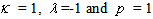 in (22) we obtain the solution
 | (23) |
Table 4 illustrates that the combined backward-Euler and rectangle rule has error O(k) for Example 2.2Table 4. Rectangle rule showing effect of time-step k, for Example 2.2, has an error of order
 |
| |
|
The last result corresponds to the simplest form of our main problem (21). In Table 4 we use the rectangle rule throughout for the integral term in equation (21). Equation (21) can be solved with the backward-Euler and Crank-Nicolson method (CN) in a similar manner. After these calculations we will extend our simple examples for more general initial conditions. First, we take the initial condition  on
on  We can obtain the exact solution for general initial conditions by using Fourier expansions.Example 2.3: Solve the problem
 | (24) |
 | (25) |
 | (26) |
The Fourier coefficient for the initial values of  is
is | (27) |
Thus  if n is odd or zero is even, giving
 | (28) |
In the following example, we have solved the equation (17) with a different initial condition. In Example 2.1, we have chosen the initial condition  however in Example 2.4, we have taken
  Example 2.4: Solve the problem
 | (29) |
 | (30) |
 | (31) |
 . If we consider the Fourier expansion of
  , then we get the solution, for
 | (32) |
where p takes odd values,  is given by
 | (33) |
Where  and
and  .The first term of (24), for p = 1, is
 | (34) |
which is  times the solution of Example 2.1, because the first term of the Fourier series of the initial condition of Example 2.4 is equal to
  times initial condition of Example 2.1. It is enough to take the first twelve terms of the solution (32), to obtain 9 figures in the results. The errors for the rectangle rule are given in Table 5. Table 5 illustrates that the combined backward-Euler and rectangle rule has error of order k for Example 2.4.
Table 5. Rectangle rule showing effect of time-step k, for Example 2.4, has an error of order

 |
| |
|
In Table 6, we used the mixed rule for Example 2.4. In this calculation, we have obtained errors of O(k). Table 6 illustrates that the combined backward-Euler (mixed rule) has error of order k.Table 6. Mixed rule showing effect of time-step k, for Example 2.4, has an error of order

 |
| |
|
3. Error Analysis in Time and Space for Backward-Euler
In this section, we introduce the discretization errors for our equation (12). In applications the operators A and B will not be differential operators such as | (35) |
But rather approximate operators (arising from finite difference space discretization) which depend on some mesh parameter h. Our results will be useful if the error bounds are uniform in h. The error at a mesh point is defined by | (36) |
As we defined in Section 2, we abbreviate  and
and  by
by  and
and  respectively. Thus
  In equation (12) replace
  by
by  giving
 | (37) |
Then it follows from (10) and (12) that  satisfy the equation
 | (38) |
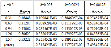
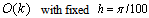
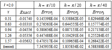
where  is the truncation error given by[3]. In Table 7, the space error is shown for the CN and trapezoidal rule (see[3] and[4]) for Example 2.1. The numerical results for the space error test give
  . The rectangle rule can be done similar manner. In Table 7, CN and trapezoidal rule showing effect of space-step for
Table 7. CN and trapezoidal rule has an error of order

 |
| |
|
In this test we see that the space error has the expected order in our numerical calculations.
4. Conclusions
In this paper, numerical method has been successfully developed for solving parabolic Volterra integro-differential equations. Numerical quadrature rules have been applied for integral term and backward-Euler method has been used for partial differential part. Errors values presented from Table 1 to Table 6 are calculated based upon backward-Euler and suitable quadrature methods with time step k. Values in these tables illustrate an error of order  . Finally, in Table 7 the space error justifies
  in our numerical solution. Numerical order of convergence is also calculated:
 We expect that Ord = 1 in time-step k and Ord = 2 in space-step h. Obtained theoretical results are confirmed by numerical experiments.
References
| [1] | Baker, C. T. H., The Numerical Treatment of Integral Equations, Claredon Press, Oxford, 1977. |
| [2] | Douglas, JR., 1962, Numerical methods for integro- differential equations of parabolic and hyperbolic types, Numer. Math., 4, 96–102. |
| [3] | Filiz, Ali, Numerical solution of some Volterra integral equations, PhD Thesis, University of Manchester, 2000. |
| [4] | Filiz, Ali, 2012, Second-order Method for Parabolic Volterra Integral Equations with Crank-Nicolson Method, Mathematica Moravica, 16-2, 13-20. |
| [5] | Linz, Peter, Analytical and Numerical Methods for Volterra Integral Equations, SIAM-Philadelphia, 1985. |
| [6] | Pao, C. V., Nonlinear Parabolic and Elliptic Equations, Plenum Press, New York, 1992. |
| [7] | Sloan, H. I. and V. Thomée, 1986, Time discretization of an integro-differential equation of parabolic type, Siam Journal of Numerical Analysis, 1052–1061. |
| [8] | Smith, G. D., Numerical Solution of Partial Differential Equations: Finite Difference Methods, Clarendon Press, Oxford, 1985. |
| [9] | Volterra, V., Theory of Functionals and of Integro- Differential Equations, Dover, New York, 1959. |
 Abstract
 Reference
 Full-Text PDF
 Full-text HTML