1. Introduction

This work is concerned with the analysis of the variation of the solution of some optimal control problems as the number of discretization points increases. For this purpose, several optimal control problems have been transcribed as constrained optimization problems which have been then formulated in AMPL language and solved considering different solvers and discretizations. To obtain results as general as possible, both elliptic optimal control problems and parabolic optimal control problems (with Dirichlet, Neumann or mixed boundary conditions) have been studied.

In Section 2 the formulation of these problems is therefore presented; in particular, elliptic boundary control problems are first described, distinguishing between the three possible cases of Dirichlet, Neumann and mixed boundary conditions. A general elliptic distributed control problem with mixed boundary conditions is then presented, followed by an example of a parabolic control problem. Eventually, some considerations on the consistency of the discretized solution with the continuous one are discussed, with particular regard to parabolic problems.

Section 3 is instead devoted to the description of the problems actually studied, which have been taken from[1], [2],[3],[4],[5].

In Section 4 the numerical results are presented and discussed. In fact, the complete results obtained with a number of discretization points ranging from 99 to 499 are reported there for every solver and for every considered discretization. The effectiveness of each solver in solving the problems is then sinthetically discussed, together with a list of the errors which more frequently occurred. Eventually, particular effort is given to the analysis of how the solution changes when the number of discretization points increases with the intent of determining if any general trend can be observed.

Finally, Section 5 summarizes the conclusions following from the analysis of the results.

2. Statement of the Problems

The formulation of elliptic boundary control problems, elliptic distributed control problems and parabolic control problems is here presented; the main references for this section are[6],[7],[1],[2].

Let be a bounded domain with piecewise smooth boundary ; the formulations of the problems are the following.

2.1. Elliptic Boundary Control Problems

The formulation of the problems is slightly different depending on the kind of boundary conditions given. In fact, the following three cases can be distinguished:

1. Elliptic boundary control problem with Dirichlet boundary conditions

(1)

subject to the elliptic state equation

(2)

to the Dirichlet boundary condition

(3)

and to inequality constraints on control and state

(4)

(5)

The functions and are here assumed to be functions.

2. Elliptic boundary control problem with Neumann boundary conditions

In this case, different boundary conditions are used and some functions are defined on different domain. In fact, the problem consists in determining a boundary control function which minimizes the cost functional

(6)

subject to the elliptic state equation (2), to the Neumann boundary condition

(7)

and to inequality constraints on control and state

(8)

(9)

where and denotes the derivative in the direction of the outward unit normal of .

The functions and are here assumed to be functions.

3. Elliptic boundary control problem with mixed boundary conditions

In this last case, even the cost function has to be written in a different way: in fact, we have to distinguish between the regions of the boundary where Dirichlet conditions are applied and the ones where we have Neumann conditions instead. The formulation of the problem is therefore the following.

Determine a boundary control function which minimizes the cost functional

(10)

where are disjoint sets that consist of smooth and connected components and such that , subject to the elliptic state equation (2), to the mixed Neumann- Dirichlet boundary conditions

(11)

(12)

and to the inequality constraints on control (4) and state (5).

The functions and are here assumed to be functions.

2.2. Elliptic Distributed Control Problem

In this case, the control function u is not on the boundary, but it is distributed in the inner space of the domain. Therefore, supposing that the boundary is partitioned as where are disjoint sets that consist of smooth and connected components, the elliptic distributed problem with Neumann and Dirichlet boundary conditions consists in determining a control function which minimizes the cost functional

(13)

subject to the elliptic state equation

(14)

to the Neumann and Dirichlet boundary conditions

(15)

(16)

and to inequality constraints on control and state

(17)

(18)

where .

The functions and are here assumed to be functions and

2.3. Parabolic Control Problem

This type of optimal control problem can be formulated as follows.

Determine a piecewise continuous function u(x,t), which minimizes the cost functional

(19)

subject to a parabolic equation, such as the diffusion-convection equation

(20)

to the initial condition

(21)

to the boundary conditions

(22)

and to inequality constraints on control and state

(23)

(24)

Both the state and the control variables are here functions of space and time. Moreover, a,b and c are known and constant parameters, with and . On the other hand, can be constant or a given function of the state y. Eventually, d is the source term, which can be a function of y, and , and are given functions which satisfy the compatibility conditions

(25)

2.4. Consistency

The solution of an optimal control problem often implies its discretization; therefore, the discretization scheme affects the solution itself and it is then important that the optimality conditions of the discretized problem reflect the ones of the continuous problem, as illustrated in[8, Chapt. 4]. It is thus important to analyse the consistency of the optimality conditions to obtain a good discretization of the problem. This can be done by considering the relationship between the Karusk-Kuhn-Tucker conditions, which constitute the discrete necessary conditions, and the continuous necessary conditions, given by the Pontryagin Maximum Principle.

For example, if we consider the parabolic problem defined by the equations (19)-(22), there must be a correspondence between the Karusk-Kuhn-Tucker equations and the co-state equations for the Hamiltonian in the Pontryagin Maximum Principle, thing that often happens when the differential equations are discretized with a difference scheme of low order[9],[10]. Moreover, in[11] the differential equation of this problem is approximated with a finite difference scheme of type FTCS, while the integrals are evaluated using the trapezoidal rule with regard to space integration and using the rectangular method for time integration; this approach results particularly suitable for the stability and the consistency of this problem.

With regard to the studied problems, necessary conditions for the elliptic problems are described in[12] and the verification of second order optimality conditions for the elliptic problems and for the first six parabolic problems is studied in[13]. It is easy to prove that the same considerations can be applied to PC_7 and PC_8 as well.

3. Description of the Problems

The following problems have been analyzed:

3.1. Elliptic Boundary Control Problems (EBC)

1. Problem EBC_1

In this problem, the cost functional consists in the tracking function

(26)

where and are given functions and is a non negative weight. Moreover, the following constraints and data are given:

2. Problem EBC_2

This problem is the same as the previous one, with the only exception that is zero instead of 0.01.

3. Problem EBC_3

The objective is always the tracking function, but the following data have been used:

4. Problem EBC_4

This problem is the same as EBC_3, but with .

5. Problem EBC_5

In this problem (and in the following EBC problems), Neumann boundary conditions have been used. The objective is here the tracking function and the following data are given:

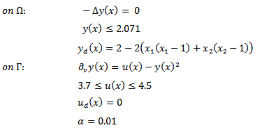6. Problem EBC_6

This problem is the same as EBC_5, but some data are different: in fact, we here have 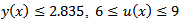and .

7. Problem EBC_7

Respect to the previous problems, the main difference is that the elliptic state equation is nonlinear; in particular, the following data are given:

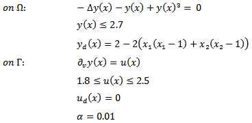8. Problem EBC_8

This problem is the same as EBC_7, but with .

3.2. Elliptic Distributed Control Problems (EDC)

1. Problem EDC_1

As in the previous problems, also here the objective is the tracking function. The following data are given:

2. Problem EDC_2

This problem is the same as EDC_1, but with .

3. Problem EDC_3

The problem is the same as EDC_1, but with different data:

4. Problem EDC_4

Even here, the only difference is that different data have been used; in particular, the main difference from EDC_3 is that we have Neumann boundary conditions in place of the Dirichlet ones:

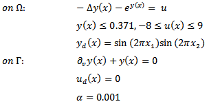5. Problem EDC_5

This problem is the same as EDC_4, but with .

6. Problem EDC_6

In this case, the objective is

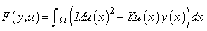(27)

subject to

1. Elliptic state equation:

2. Omogeneous Neumann boundary conditions:

3. Constraints on control and state:

Moreover, the following numerical values are given:

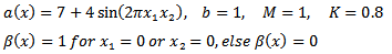
3.3. Parabolic Control Problems (PC)

1. Problem PC_1

The cost functional is here given by

where and it is subject to

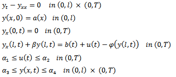where:

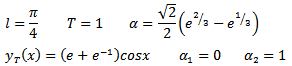
2. Problem PC_2

The problem is the same as PC_1, but with the following numerical data:

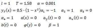3. Problem PC_3

The only difference from PC_2 is that here we have and

4. Problem PC_4

This problem is the same as PC_3, but with and

5. Problem PC_5

This problem is the same as PC_2, with the following differences: we here use the nonstationary Burgers equation with , and we have and

6. Problem PC_6

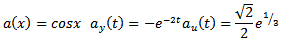
PC_6 is the same as PC_2, but with and .

7. Problem PC_7

This problem is based on the river aeration problem presented in[4], where more detailed information about the model and the variables are provided. The objective is:

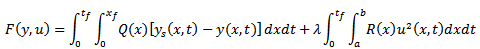where the control variable u is the rate of aeration, the state variable y is the concentration of dissolved oxygen, y_s represents the saturation value of dissolved oxygen (here assumed constant and equal to 6 mg/l), while Q(x) and R(x) are weight functions assumed to be equal to 1, just like which is a scalar parameter.

The objective is subject to the following constraints:

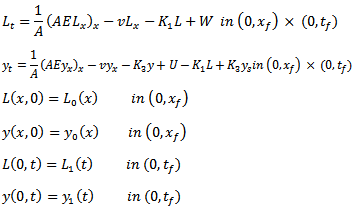where L is the biochemical oxygen demand and W is the discharge rate of the biochemical oxygen demand (assumed constant in the analysed problem). Moreover, neglecting the tidal action and assuming constant the cross sectional area, the problem can be simplified by omitting the terms and .

Finally, the following numerical data are given:

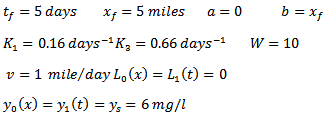8. Problem PC_8

PC_8 is based on[5] and regards the problem of firing industrial kilns according to a given reference profile. The objective is:

where y(x,t) is the state variable, u(t) is the control, T = 0.7 and p(t), in the numerical example considered, is given by:

Moreover, the following constraints are given:

where:

4. Results and Analysis

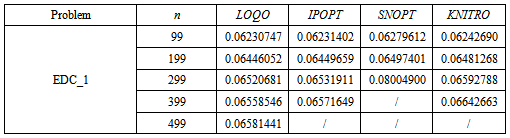
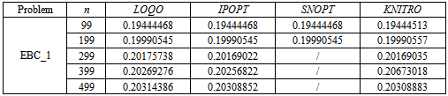
The following results have been obtained by writing the previously presented problems in AMPL language and by solving them with different solvers and number of discretization points. In particular, the problems have been solved through the NEOS servershttp://www.neos-server.org/neos/[14],[15],[16] by calling the solvers MINOS[17], KNITRO[18], IPOPT[19], LOQO [20] and SNOPT[21], [22].

As regards the discretization, the elliptic problems and the first six parabolic problems have at first been solved with discretizations based on the codes in[23]. Therefore, the elliptic problems have been discretized with the composite rectangle rule to approximate the integrals and with simple discretization techniques (such as the five-point stencil and the Euler method) to approximate the derivatives, while in the first six parabolic problems and in PC_8 the composite trapezoid method, the Crank-Nicolson method and a second-order three-point formula derived from the method of undetermined coefficients have been used. On a second stage of the analysis, other discretizations have then been analysed, as described later in this section.

PC_7, instead, has been discretized by using the FTBS (forward time backward space) method for the formulation approximate the integrals; moreover, being the used method explicit, the stability criterion for the method itself has been verified before computing the solution.

In Table 1, then, the results obtained for the problems discretized as described before are presented. The solutions computed by MINOS are not reported since the solver has been able to solve only a few problems, due to the relatively high minimum number of discretization points considered; a short comment on the behaviour of MINOS and of the other solvers is however given after Table 1.

Moreover, it has to be noticed that whenever a second discretization index m was required, it has been set equal to n; for this reason, the only discretization index reported in Tabel 1 is n.

Table 1. Results for the Minimum of the Objective for Different Solvers and Discretization Points

To enhance the table readability, it has been chosen not to write in the table the kind of error that has been encountered every time the solver was not able to solve the problem, but simply to mark the corresponding box with a slash; the most common errors encountered with each solver are therefore here synthetically described.

MINOS was found not to be fit to solve the vast majority of the problems (even if, actually, it has been possible to solve several problems lowering the number of n below 99, which, however, is the minimum number of discretization points considered in this work). The most common errors are infeasible problem, infeasible problem (or bad starting guess), too many major iterations, singular basis after several factorization attempts and unbounded (or badly scaled) problem.

The most common errors in LOQO are due to the exceeding of the iteration limit, set to a maximum of 500 iterations, and of the time limit (even though this error occurred more rarely and only for large numbers of discretization points). The reaching of the iteration limit, however, does not mean by itself that the computed solution is far from the real one, since the solver could be near to the convergence to the solution when the limit of 500 iterations was reached; therefore, even when this error occurred, sometimes LOQO computed acceptable solutions, consistent with the ones computed by the other solvers.

In IPOPT the most frequently encountered error is not enough memory. Moreover, it has been encountered twice also the error converged to a locally infeasible point. Problem may be infeasible. In particular, this happened in EBC_7 and EBC_8 for n=199, where SNOPT converges to the same infeasible point too.

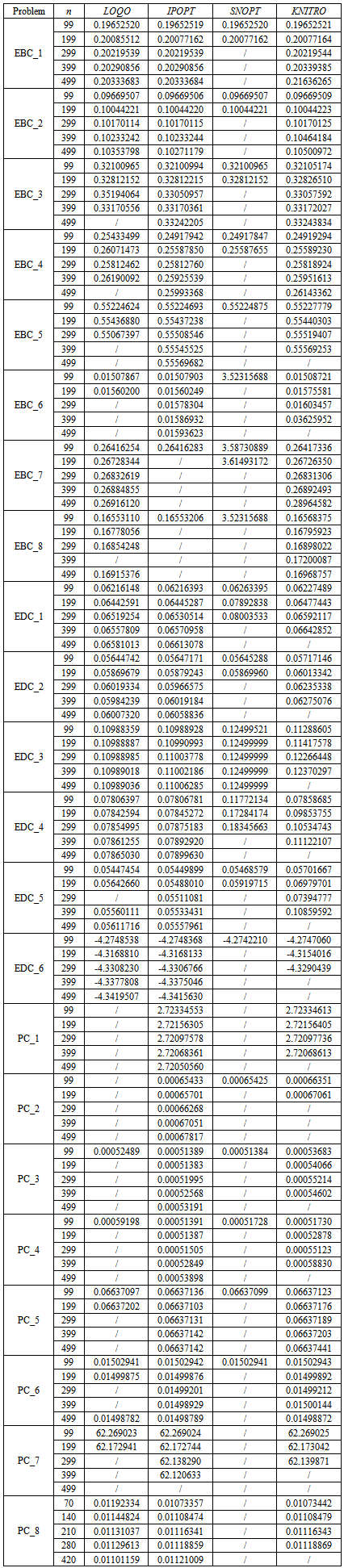
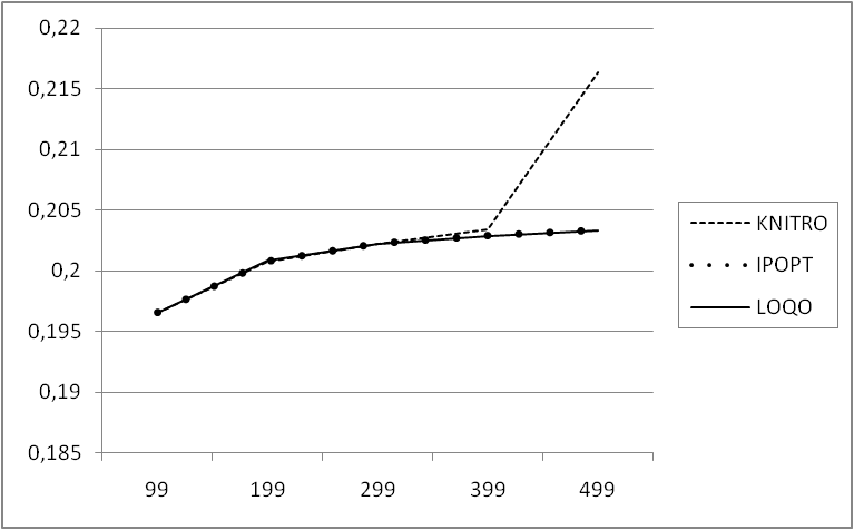Figure 1. Results for the minimum of the objective for EBC_1

As mentioned in the previous paragraph, SNOPT sometimes computes a solution not in line with the ones computed by the other solvers, as it can be seen in Table 1; moreover, the following errors have often occurred: not enough real storage, not enough integer storage and time limit reached.

Eventually, the most common error encountered in KNITRO is not enough memory.

As regards the variance of the minimum of the objective as the number of discretization points increases, it must be distinguished between elliptic and parabolic problems.

As for the elliptic problems, the value of the objective tends to increase (in absolute value) as the number of discretization points increases, as shown in Table 1. This trend, though, sometimes is not verified for large numbers of discretization points (in fact it is not always possibile to find a definite trend over 399 points). 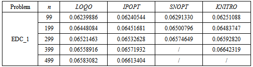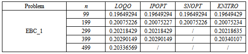Notwithstanding this, every analysed problem shows an increasing trend at least for for every solver able to properly solve the problem itself. Moreover, even when the increasing trend is not respected in one solver, it is generally so in the others (see Figure 1). Therefore, even if, on one hand, the influence of the solver on the solution seems to be negligible in the vast majority of cases (since the solution often presents only small variations), on the other the analysis of the consistency of the solution between different solvers is of the utmost importance to detect possible out-of-range values.

Instead, it is not possible to find any general trend for the parabolic problems: in fact a decreasing trend can be observed in some cases, but it does not happen always, even for a number of discretization points significantly large.

Therefore, it appeared more interesting to deepen the study of elliptic problems by verifying if the observed trend is dependent on the type of discretization used; to do so, the elliptic problems have been solved again using different interpolation formulas to approximate the integrals. In particular, while the results reported in Table 1 have been obtained using the composite rectangle method, the ones in Table 2 and in Table 4 have been calculated with a different kind of composite rectangle method, hereafter referred to as Composite Rectangle Method - B, evaluating the function on the right bound of each interval rather than on the left one. Eventually, the results in Table 3 and in Table 5 have been obtained using the composite trapezoidal rule.

Table 2. Results Obtained for EDC_1 Discretizing the Integrals with Composite Rectangle Method - B

Table 3. Results Obtained for EDC_1 Discretizing the Integrals with the Composite Trapezoidal Rule

Table 4. Results Obtained for EBC_1 Discretizing the Integrals with Composite Rectangle Method - B

Table 5. Results Obtained for EBC_1 Discretizing the Integrals with the Composite Trapezoidal Rule

Every elliptic problem has been solved with both these discretizations; however, since the solutions are really similar to the ones already reported in Table 1, it has been chosen to present only the results concerning two case problems. The results and the analysis hereafter produced are therefore to be intended as referred to the whole set of elliptic problems and not to EBC_1 and to EDC_1 only.

The tables presented confirm the results previously observed: in fact, though of course there are some differences due to the different discretizations used, the increasing trend is preserved. Therefore it can be concluded that this trend does not depend on the type of discretization used.

It is also worth noticing that the discretization with the trapezoidal rule resulted more stable than the other interpolation formulas: in Table 4, in fact, it can be noticed that for n = 399 KNITRO computes a solution which, although it is not so far from the expected value, is larger than and not completely consistent with the solutions computed by LOQO and IPOPT for the same number of discretization points; because of this, the result computed by KNITRO for n = 499 is lower than the one for n = 399, while in the other solvers the increasing trend is preserved. In Table 5, on the other hand, the solutions show a more regular increasing trend, without any value out of range. This also happens in other problems and, therefore, not only the trapezoidal rule appears to be more stable but the increasing trend is also preserved more often than with the other discretizations. However, it has also to be noticed that the use of the trapezoidal rule also leads to a more complex formulation of the problem, and because of this in Table 5 (and in a lot of other problems discretized this way) it has not been possible to find the solution for n = 499 with the solvers IPOPT and KNITRO.

As regards the errors occurred, the same considerations made for Table 1 apply; the only thing that can be noticed is that the error Time limit is more frequent in solving the problem with the integrals discretized with the trapezoidal rule due to the greater computational complexity of the method itself. For the same reason, also the error not enough memory occurs more frequently and for lower numbers of discretization points.

5. Conclusions

The results presented and analysed in the previous section allow to come to the following conclusions:

1. As for elliptic problems, it is possible to identify an increasing trend of the absolute value of solution as the number of discretization points increases. This trend can be observed in every elliptic problem studied for a number of discretization points n lower than or equal to 299. Instead, for n = 399 and for n = 499 the trend may or may not be respected for some solvers.

2. The use of different solvers or of different interpolation formulas to approximate the integrals of the objective changes the value of the solution, yet it does not influence the trend described in the previous point.

3. It is not possible to identify any general trend as regards the parabolic problems: in fact, in PC_1 and in PC_7 the solution decreases as n increases, while in other problems an increasing trend is observed and in others it is not possible to identify any trend at all.

4. Regarding the parabolic problems, the trend can be dependent on the solver used: for example in PC_4 the solution computed with KNITRO increases, while the one computed with IPOPT at first decreases and then increases. In general, the solutions computed with KNITRO tend to increase as n increases for n ≤299 with the sole exception of PC_1, while IPOPT has less regular trends and the other solvers are often not able to properly solve the problem.