Paul T. R. Wang, William P. Niedringhaus, Matthew T. McMahon
The MITRE Corporation, Center for Advanced Aviation System Development (CAASD), 7515 Colshire Drive, McLean, Virginia, 22102-7539, USA
Correspondence to: Paul T. R. Wang, The MITRE Corporation, Center for Advanced Aviation System Development (CAASD), 7515 Colshire Drive, McLean, Virginia, 22102-7539, USA.
| Email: |  |
Copyright © 2012 Scientific & Academic Publishing. All Rights Reserved.
Abstract
The authors illustrate the use of new algorithms for solving the feasibility problem ofsystems of linear inequalities in variables that define location, distance, speed, and time between aircraft in 4D space to achieve the desired aircraft movement obeying safety separation, speed limit, air traffic control restrictions, and desired flight path. This new linear inequalities solver (LIS)technique is applicable to any system of linear inequalities including linear programming, eigenvector programming, and systems of linear equalities. The three new LIS algorithms are: 1)Simplex alike method to reduce the worst infeasibility of a linear system, 2) a zero-crossing method to reduce the sum of all infeasibilities of a given linear system, and 3) a de-grouping algorithm to reduce the size of the set of constraints with the worst infeasibility,These set of new LIS algorithms were coded in Java and tested with MITRE CAASD’sairspace-Analyzerwith hundreds of aircraft over thousands of variables, and tens of thousands of linear constraints. At high precision, solution of the LIS matchesthesolution obtained from the same LP problem using conventional Simplex method and methods used by Cplex, GNU LP solver, etc. The advantages and challenges of this generic LIS versus known, well-established algorithms for linear inequalities are also discussed.
Keywords:
Solution of Linear Inequalities, Algorithms, Air Traffic Control, Homogeneous Linear System, Self-dual Formulation, Linear Infeasibility, etc
Cite this paper: Paul T. R. Wang, William P. Niedringhaus, Matthew T. McMahon, A Generic Linear Inequalities Solver (LIS) with an Application for Automated Air Traffic Control, American Journal of Computational and Applied Mathematics , Vol. 3 No. 4, 2013, pp. 195-206. doi: 10.5923/j.ajcam.20130304.01.
1. Introduction
The authors present new concepts and algorithms to solve any system of linear inequalities in homogeneous form, which includes linear programs, eigenvectors, orthogonal space, and systems of linear equalities or inequalities. Four key algorithms were developed, coded, and tested to reduce the worst case of infeasibility, sum of infeasibilities, and the number of constraints with the worst infeasibilities. This paper is organized into the following 10 sections:Section 2. Linear Systems Feasibility (LSF)Section 3. An Airspace Analyzer using LPSection 4. A Simplex alike method Section 5. Zero-crossing in LSFSection 6. De-grouping the worst infeasibility setSection 7. Convergence/Completeness Analysis Section 8. Decomposition and Combinationof LISSection 9. LIS ScalabilitySection 10. Advantages and ChallengesSection 11. Conclusion and Future Work
2. Linear Systems Feasibility (LSF)
Given any system of linear inequalities or equalities in vector and matrix form,  where
where  is an m by n matrix,
  and
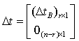
and  are n by 1 column vectors.We define the linear systemfeasibility (LSF) for
  as follows
 where
where | (1) |
The vector  is referred to as the feasibility vector of the original linear system of inequalities
 .
.
2.1. A Literature Overview and Motivation
Traditionally, linear inequalities are resolved as linear programs using either the Simplex methods[1][2][3] &[4], Crisis Cross algorithms[5], interior point method[6] projective algorithms[1][7], path-following algorithms[8], andpenalty or barrier functions[9]. Most approaches centered on iterative searching for feasible points within the polytope defined by the constraint linear inequalities. The authors propose a new approach that recursively reduces the worst infeasibility, the sum of all infeasibility, and the number of constraints with the worst infeasibility based upon nonzero coefficients or a subset of the nonzero coefficients that defines the given system of linear inequalities. Such an approach is capable of finding the exact solution if such a feasible solution is unique, a feasible solution if there are more than one solution. For linear system that does not have a feasible solution, this approach is capable of minimizing the sum of all infeasibility or the worst infeasibility, and pinpointing to the relevant coefficients to reveal true conflicts of the linear system.
2.2. Overview of New Algorithms to Minimize Linear Systems Infeasibility
The feasibility vector of a linear system,  in (1) provides new algorithms that can be used to minimize the sum of all infeasibilities as
  for all the infeasible rows, the worst infeasibility,
  , or the number of constraints (rows) with the worst infeasibility as the set size of
  . This set of new algorithms may be applied recursively based upon their maximum possible gains at a given step. All algorithms are built upon the non-zero coefficients of a given linear system and extremely efficient for very large sparse linear systems. Figure 1 illustrates the overall concepts of this recursive liner infeasibility reduction strategy using the key three algorithms presented in this article.
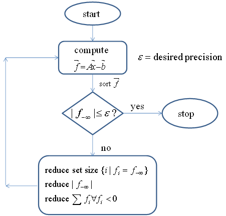 | Figure 1. A Recursive Strategy to Minimize Linear Infeasibility |
3. The Airspace Analyzer Application
The MITRE Corporation’s Center for Advanced Aviation Development (CAASD) has developed a tool, airspace - Analyzer (aA)[13][14], which simulates automated air traffic control (ATC). It separates traffic while respecting aircraft performance and ATC restrictions and procedures (REFs). We test the LIS algorithms using LPs generated by airspace-Analyzer, which for the entire continental US airspace (3000 simultaneous aircraft) typically have several hundred thousand variables and about a million constraints.At each tick of its simulation clock, airspace-Analyzer iterates the following steps:(a) Resolve the scenario at the current simulation time, looking out into the future to some time horizon (typically six minutes). (b) Advance the simulation clock by a fixed time-increment (typically two minutes)(c) Incorporate any resolution maneuvers requiring changes in aircraft positions at the new simulation time.The inputs are the planned (X, Y, Z) positions of each aircraft at future times, along with restrictions and airspace parameters. Airspace-Analyzer represents the (x, y, z) positions of each aircraft at future times as variables in a linear program (LP). These match the input (X, Y, Z) unless a maneuver is needed, e.g. for separation vs. another aircraft. The LP’s constraints represent ATC constraints—on aircraft performance, permissible altitudes and speeds, and sufficient vertical or horizontal separation for each pair of aircraft Some of these are nonlinear, but can be approximated linearly (so that they are made more, not less, stringent). The LP’s objective function maximizes forward progress, less certain weighted penalties discussed below.The LP is designed to always be feasible, even though there might not be enough airspace to meet all ATC restrictions. For instance, suppose Aircraft A should be at or above 25000’ t t=5. This could be expressed as “zA,5>=25000”. However, traffic might be so dense that safe separation is inconsistent with this constrait. To assure LP feasibility, this constraint (say, the i-th) is represented as: “zA,5>=25000 - di”, where di is a new (nonnegative) LP variable. To drive the value of di to 0 when possible, a term Cidi is subtracted from the objective function. The value of the constant Ci reflects the importance of driving this di to 0, relative to other “d” variables for other constraints. Separation constraints would have the highest value for C (virtually infinite). The LP typically includes constraints specifying desirable but non-essential ATC features (e.g. “keep the maneuvers simple”), with C values lower than those specifying ATC restrictions.The full airspace-Analyzer LP will be published in a future paper. A simplified form appears in[13]. An even simpler version suffices here; it provides speed and separation constraints for a two aircraft in the horizontal dimension only. Aircraft are modeled to fly along trajectories, which are sequences of points (called cusps) in xyzt-space. Between consecutive cusps, aircraft are assumed to fly in piecewise linear segments; maneuvers (turns, speed changes, vertical maneuvers) occur only at cusps. A simplifying assumption is made that maneuvers are instantaneous, so that one may interpolate along such segments to find the aircraft's continuous positions in xyzt-space at times between two consecutive cusps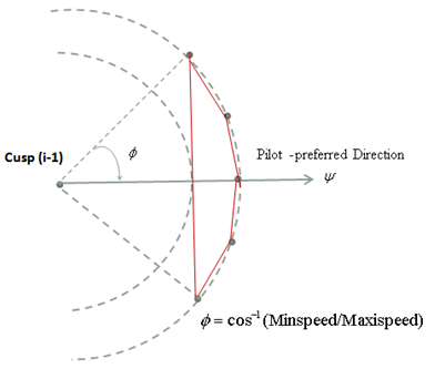 | Figure 2. Defining A Feasible Region Between Aircraft |
Figure 2 shows an aircraft moving in direction  (eastbound in the figure) between Cusp (i-1) and Cusp (i). It is modeled as being able to make an (instantaneous) turn right or left by a maximum angle of
  at Cusp (i-1). It then flies linearly at a speed that can range from minSpeed (inner circle) to maxSpeed (outer circle). We can define Φas:
 The region between the two circles (possible positions for Cusp (i)) is nonlinear and nonconvex, but a useful subset of this can be bounded by a convex 5-sided polygon. The inequality for the long side of the polygon in Figure 2 is
 Inequalities for the four short sides of the polygon are then:
 where:
3.1. Separation Inequalities
To define (horizontal) separation inequalities, it is useful to consider the aircraft in relative rather than absolute space. Figure 3 (a) and (b) show an example 90° encounter between Aircraft j and k, in absolute space and relative space, respectively. In Figure 3 (a), Aircraft j flies north, passing ahead and to the right of the eastbound Aircraft k. In this example there are four segments (M = 4). The nominal positions of Cusp (i, j) and Cusp (i, k) are shown for i = 0, 1, 2, 3, and 4, assuming j and k ignore each other and fly their preferred (straight) route. In Figure 3 (b), a coordinate transformation is applied, so that Aircraft j's position is fixed at the origin (for i = 0, 1, 2, 3, and 4). Aircraft k is seen to be moving southeastward relative to j. Note that the vector from j's i-th cusp to k's i-th cusp, for all values of i, is the same in both Figure 3 (a) and Figure 3 (b).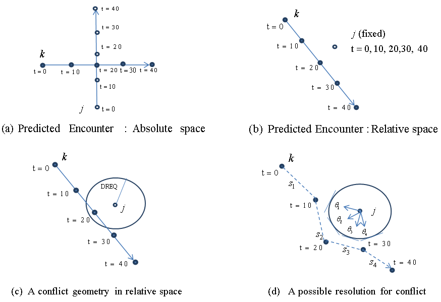 | Figure 3. Two Aircraft Encounter and Their Separation |
In Figure 3 (c), a circle is drawn around j's position with radius equal to the required separation distance (denoted DREQ). Aircraft j and k are separated by at least DREQif and only if k's segments in relative space all stay outside the circle. The task here is to so specify, using only linear inequalities/equalities in the airspace-Analyzer variables.Airspace-Analyzer's means for asserting in its LP that the Figure 3 (c) aircraft are always safely separated is shown in Figure 3 (d). The four segments of k are labeled  , for i = 1, 2, 3, and 4. Points are shown on the circle. If for each i,
  is on the opposite (safe) side of the circle from a line tangent to the circle at then Si never enters the circle, so k never enters the circle, and is safely separated at all times from j.To assure that the i-th segment of Aircraft k in relative space is on the proper (safe) side of the tangent line at
  it is necessary only that the beginning and ending cusp are on the proper side. The following pair of linear inequalities is satisfied if and only if the two endpoints of segment Si are entirely on the safe side of the tangent line at
  :
:

3.2. Spacing Inequalities
airspace-Analyzer also allows two aircraft (j and k) to be given a miles-in-trail (MIT) constraint. That is, they are to be spaced a certain distance at a certain time by a certain distance. For instance, if j is supposed to be 10 MIT ahead of k in the eastbound direction at time i, the inequality isxi,j – xi,k>= 10.
3.3. Additional Constraints Needed to Achieve air Traffic Control Objectives
Many other constraints are used in airspace-Analyzer, to accomplish a variety of air traffic control goals. Examples include:− Altitude Restrictions (e.g. an aircraft reaching a certain position should be at or below a specific altitude)− Sector Boundaries (e.g. an aircraft should stay within its sector until its planned exit position) − Simplicity (Suppose an aircraft’s trajectory has four segments (as in Figure 3). If the first two and the last two are collinear the maneuver is simpler than if not. It is possible to extract a small penalty for a solution that fails to make them collinear.
3.4. One-aircraft and Two-aircraft Constraints
For the purposes of this paper, it is sufficient to know that speed constraints (from Figure 3-1) and the constraints of Section3.3 reference only a single aircraft. The only constraints that refer to more than one aircraft are separation and spacing constraints; and they refer to exactly two aircraft.In our decomposition strategy, we refer to the subset of constraints that reference exactly one particular aircraft as the “atomic” LP for that aircraft. In 3D, separation is accomplished by separating trajectory segments from a cylinder or ellipsoid by tangent planes. Niedringhaus’s 1995 IEEE paper[13] provides additional details.
4. A Simplex alike Method to Reduce 
In this section, we illustrate how an ordinary linear program (LP) may be converted to a s Linear System Feasibility (LSF) problem such that a technique similar to the Simplex method used in linear programming is applied to reduce the worst infeasibilitiesfor a small selected subset of the linear constraints of a given LSF.
4.1. Self-Dual LP as LSF
For a given linear program (LP),boththe primal and dual LPs may be combined into a self-dual LP so that the dual is the same as the primal and the objective function becomes simply a pair of linear inequalities. Converting LPs into self-dual form, we can enforce homogeneity with one additional dimension as:The primal LP:  The dual LP:
  Optimality:
  The self-dualLP as LSF[15][16]:
 | (2) |
Note that solution to the self-dual LP as LSF implies both primal and dual feasibility of the original LP. In other words,a feasible self-dual LSF enforces optimality for the original LP with the primal objective equal to the dual objective, i.e.,  .Inequalities (2) is only one of many possible LSF for an LP, alternatively LSF formulation for LP with different primal and dual variable bounds do exist.Applying row permutation to an LSF such that the feasibility vector, f, is sorted in descending order. In other words, rows in Sare regrouped into four distinct sub-matrices such that all the rows with positive feasibility (
 ) are in
 , all the rows with zero feasibility (
 )are in
 , all the rows with the worst infeasibility (
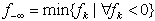 ), are in
 , and the rest of rows (
 )are in
 .
. | (3) |
Note that all rows in  have the same worst (or maximum) infeasibility
 .
.
4.2. ASimplex alike Method for 
The Simplex method is used to solve either the primal or the dual LP. To apply the Simplex method, one starts with the identity matrix as a basis matrix for all the column variables. A basis matrix with its rank equal to the total number of column variables is maintained by exchanging some or all of the basis columns and rows with non-basis rows or columnsFor the LSF, the feasibility vector is sorted in descending order with respect to its feasibility. We apply a technique similar to the Simplex method only to constraints with the worst infeasibilities,  . The following recursive procedure is used to assure that the set of constraints with the worst infeasibilities is always full ranked and the set size of
  is kept as small as possible.Note that the size and row indices for the worst infeasibility,
  changed from one step to the next, hence, the Simplex method is not directly applicable; however, we can use the same technique inverting a nonsingular basis matrix for the rows in
  to compute an adjustment to the vector ,t, as
  such that the infeasibility for all the rows in
  are reduced simultaneously and equally.Sort feasibility,
  , for rows in
 ,as
,as .Let
.Let
 While (0 <k-r){Replace set
  by the set of rrows in
  with the same worst infeasibility.Computek and r.}Note that the worst infeasibility for rows in
  are subjected to errors in rounding and truncations; gaps between rows may be scaled to magnify their difference. A LSF scaling algorithm is provided later in Section 9.Once we have a full-ranked
  , the following steps are used to reduce the worst infeasibility
  . The superscription, C, is used to denote the complement of a sub matrix.
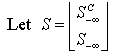 | (4) |
and assume that  is full ranked with r rows; i.e., we have
 | (5) |
We can perform column permutations to rearrange columns of  as:
as: | (6) |
Where  is a nonsingular square submatrix of
 .Any adjustments as shown in Figure 3 to
  may be treated as the results of multiplying
  by
by  ,
,  | (7) |
Hence, for any  , we have
  | (8) |
Let  where
where 
 | (9) |
 | (10) |
 | (11) |
Although  does remove the worst infeasibility
 for all rows in
  as shown in Figure 3, its impact on other rows in
  cannot be ignored. For each row,
  in
in , let
, let | (12) |
Applying  to
to  at row i, we obtain
  | (13) |
Note that the necessary conditions for  to be beneficial are
  and
and  . Solving for the maximum possible
  , we have.
 | (14) |
Note that from Figure 4,  is where
  meets
meets  with
with  applied.From Figure 3, the row in
  with the smallest
  is the maximum improvement
  can be achieved with
 . Hence,
  | (15) |
In summary, this algorithm deals with all the rows in . Similar to the Simplex method, a small adjustment,
  to the tentative solution, t, is computed from the full-rank basis for all the rows in
  . All the rows in
  are decomposed into
  while
while  has the same row rank as that of the
  . Let B be a nonsingular square sub-matrix of
  such that
  . The basis matrix, B, may be constructed from
  by sequentially selecting linearlyindependent columns. Alternatives to pick linearly independent columns from
  as a basis matrix B does exist.Similar to the Simplex method, we compute the maximum allowable adjustment to
  as follows:
  while
while  with
with  , where
  .Comparing to the Simplex method that operates on a full size nonsingular basis for the constraint matrix, A, this Simplex alike basis matrix, B, is only a very small subset computed from the linearly independent rows in
  . In summary, the following three steps are applied recursively to reduce the maximum infeasibility,
  Step 1. Assume that
 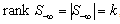 , selectk linearly independent columns from
  such that
 where B is a square non-singular sub matrix of
  .Step 2. Compute the maximum possible reduction of the worst infeasibility
  for
for  as
as 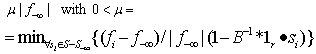 Step 3. Adjust the vector
  Steps 1 to 3 to reduce
  may be applied recursively.Figure 4 illustrates the maximum possible reduction of the worst infeasibility using this Simplexalike method. Note that the basis matrix is obtained from a small subset of all the rows (with the maximum infeasibility) and that its rank varies from one step to the next as the landscape of the feasibility vector,
  changed from one step to the next.Figure 4 also illustrates the fact that utilizes the basis matrix for rows in
  to reduce simultaneously the value of
  may be bounded by a potentially blocking row, b,with its feasibility
 such that
 with
with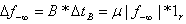 .
. | Figure 4. A Simplex Alike Method for  Reduction Reduction |
5. Zero-crossing in LSF
The second algorithm utilizes nonzero coefficients of a given LIS to identify zero-crossing points for the LIS such that the sum of all infeasibilities may be reduced. Note that reducing the sum of all infeasibilities may or may not result in the reduction of the maximum infeasibility ( ). For an infeasible row (such as row i) to become feasible, one must adjust the feasibility
  through a nonzero coefficient,
  of a related column, j, of row of
  . Such nonzero column of
  defines the set of all-zero crossingsfor
  . This algorithm identifies all the zero-crossing points for S and tests their impacts on both the sum and maximum infeasibility for S. Among all possible zero-crossing points, one can identify columns that can be used to maximally reduce the sum of infeasibilitiesover all the infeasible rows. Simply stated, this algorithm computes the difference in the sum of infeasibility for every nonzero column coefficient at its zero-crossing points for any infeasible row.Each nonzero coefficient associated with an infeasible row uniquely defines such a zero-crossing opportunity. Let
  be the sum of all infeasible rows of f, any nonzero coefficient,
  at row icolumnu provides a zero crossing point for an infeasibility row,
  , with adjustment of column variable,
  such that,
 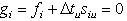 . Such a zero crossing point for
  will have it global implication on the new sum of all infeasibility rows. In other words, the new infeasibility sum will be
  . Consequently, we will have a net gain or loss of the infeasibility sum for the feasibility vector, f, as
  . i.e.,
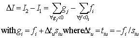 | (16) |
 | Figure 5. Reducing the Sum of Infeasibility with Zero-Crossings |
The maximum number of possible zero-crossing points is equal to the total number of nonzero coefficients in S. One can easilyidentify a zero crossing point that yields the maximum  .This algorithm may be applied recursively to reduce the sum of all infeasibilities of S until no further reduction exists. Figure 5 illustrates the reduction of the sum of all infeasibilities of S or the size of
  or both for a non-zero column coefficient,
  or
or .
.
6. De-grouping the Set of Rows with the Worst Infeasibility
This Simplex alike method is capable of recursively reducing the magnitude of the maximum infeasibility,  . Applying the zero-crossing for infeasible rows is capable of recursively reducing the sum of infeasibilities for all rows. It is likely that the set size of
  may increase noticeably. An algorithm is needed to reduce the set size of
 . This is accomplished with columns that are reachable from rows in
 . If a column, j, reachable (with non-zero coefficient,
  ) by the rows in
  has row coefficients for those rows are of the same sign (either positive or negative), then one can reduce the set size of
  by moving up those rows from the set of
  since the infeasibility of all those rows may be reduced concurrently by adjusting the column variable in the beneficial direction, i.e., positive or negative, as shown in Figure 6. Simply stated, the following steps are identified to recursively reduce the number of rows with the worst infeasibility,
  , in any LIS:Step 1: Determine the set of all rows with the worst infeasibility
  :
:  Step 2: Determine the columns that are reachable from any rows in
  :
: 
 | Figure 6. De-grouping the  |
Step 3: For each  in
in  determine all the rows in
  that are reachable from
  Step 4:Check if all rows in
  are of the same sign (positive or negative)Step 5: If
  is of single sign, the size of
  can be reduced by the size of
  In other words: adjustment of variable for column
  will reduce the size of
  by the size of
  (
( )
)
7. Convergence/Completeness Analysis
Theconvergence of the proposed LIS algorithms, namely, the Simplexalike method to reduce  , zero-crossing to reduce sum of infeasibility, and de-grouping to reduce the set size of rows in
  may be illustrated with the following arguments:Let t be a feasible solution for
  if such feasible solution does exist, and x be any vector such that
 . Sort the vector g in descending order as
 | (17) |
Note that we have , there are only three cases:Case 1:
  with
with  Case 2:
  with
with  andCase 3:
  For Case 1, the vector (t-x) reduces
  for all rows in
  , Hence, the economical Simplex method has nonzero solution.For Case 2,
  is unchanged, however,
  is reduced by the vector (t-x). Hence, de-grouping has no trivial solution.For Case 3, we have
  , hence the vector (t-x) must reduce the sum of infeasibilities for g. Since all adjustments to x for g are the zero-crossing points, at least one such point must reduce the sum of infeasibilities in g. Hence, zero-crossing willhave nonzero solution. Consequently, we can always find an adjustment to x as
  from g and t such that
  has either a smaller
  (larger minimum g), or a smaller
  , or a smaller sum of infeasibilities.
8. Decomposition, Combination, and Scalability of LIS
It is possible to decompose a given LIS into two coupled LISs with row and column permutations. The children LISs can then be solved in parallel. The solution of the parent LIS is then obtained with minimum changes to the combined solutions of the children LISs and the combined column variables. Figures 7 and 8 illustrate this LIS decomposition and recombination relation that can easily be implemented in any parallelcomputing platform.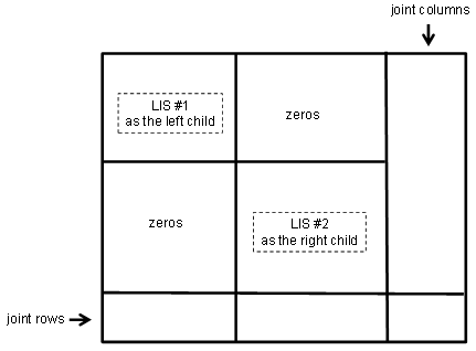 | Figure 7. A Binary Decomposition of LIS |
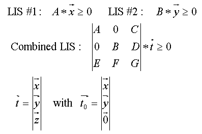 | Figure 8. Combining Two LISs |
9. LIS Scalability
The following analysis illustrates the scalability of LIS with respect to the solution vector. Scalability can be utilized to separate true infeasibility gaps from the errors of rounding and truncation. Consequently, scaling LIS can result in higher precision and fast convergence.Assume that one wishes to solve  at
at  If we solve
  at
at , we have
 at
at  Consequently, achieving worst infeasibility at
  for g is the same as achieving
  for f. The scaling of the vector b has the effect of magnifying the infeasibility gaps with the same scale. A very large scaling factor for b can magnify the infeasibility by the same scale and hence decoupling ordinary rounding and truncation errors from the true infeasibility gaps. Experiments with Java code has confirmed this observation and significant reduction in run time was also observed with very large LIS scaling factor of
  for CAASD’sairspace-Analyzerapplication.
10. Advantages and Challenges of LIS in LSF Form
In summary, the authors have shown that converting ordinary system of linear inequalities to its feasibility form, LSF, offers the following advantages:• LSF may be solved with three new algorithms that recursively reduce the sum of infeasibility of all constraint inequalities, the maximum infeasibility among all the linear constraints, and the number of constraints that share the same worst case infeasibility. Each algorithm is shown to utilize CPU time that is proportional to the number of nonzero coefficients (NNZ) of a small subset of all the nonzero coefficients of the constraint matrix, A, that defines the system of linear inequalities. • LSF can be solved with recursive binary decomposition and recombination for very large number of variables and constraints in the range of tens of thousands.• LSF covers all linear systems including system of linear equalities (singular or non-square systems included), liner programs formulated in self-dual form, eigenvector program, bounded linear systems, orthogonal vectors, and ordinary system of linear inequalities.• LSF provides a simple scaling capability that can be used to improve the precision and speed of its key algorithms.• LSFcan easily be implemented in a parallel computing platform to take advantage of concurrent CPU, multi-threading, and the advantage of Graphics Processing Unit (GPU) computing.Initial tests with hundreds of large size sparse LPs from scenarios generated by CAASD airspace-Analyzer(aA) clearly demonstrated these advantages. As shown in Figure 7, LIS can recursively obtain a feasible solution of a given system of linear inequalities in LSF form from the solutions of it components as a left and a right child LSF with only minor changes to the combined solutions such that to remove infeasibility that is purely the results of additional nonzero coefficients in both the joint rows and joint columns.Hence, one would expect that LIS will be very fast for applications that are very sparse with small size of joint rows or columns for the parent node of its left and right child nodes. We have coined such applications as “LP local” to reflect the following two properties: Its sparsity increases with size and its optimal cut set of its left and right children has a small number of joint rows or columns. CAASD’s aAhas been shown to be a good example of such LP local applications. We have testedvarious scenarios of aA for up to 3200 aircraft with 0.2 million variables (columns),0.5 million constraints (rows), and 2.3 million nonzero coefficients (NNZ) of the LSF.Initial experimental timing profiles using both LIS and GLPK for the entire continental UStest cases as 13 level decomposed binary trees shows that GLPK has a timing profile slightly better than the  where n is the number of variables (columns) and LIS without threading, GPU, or parallelization has a timing profile that is slightly worse than
  wherem is the number of constraints (rows) and
  is the sparsity of the constraint matrix, A. Using MITRE CAASD application airspace-Analyzer as a linear program (LP) for conflicts resolution and operational constraints for the entire continental US with ¼ million variables, ½ million constraints, and 4 million NNZs, the experimental results as shown in Figure 9 shows that the computational complexity of LIS is slightly worse than
  We also show that with latest GLPK 4.47 over CAASD 40MB Linux 64-bit computers, the same LP can be solved with a computational complexity that is slightly better than
  . Figure 9 illustrates the difference in computational complexity obtained experimentally with both LIS and GLPK. First, the aA application as a single linear program (LP) that handles all 3400 aircraft for the entire US National Airspace (NAS) is formulated as the root node of a 13 level binary tree. The LP represented by a parent node on such a binary tree is then decomposed into a pair or left child and right child nodes as depicted in Figure 7 such that we have minimum number of joint rows, joint columns, or joint NNZs. Such binary decomposition is carried out using optimal or near optimal cutset algorithm METIS software. Each node over this binary tree is further decomposed recursively into pairs of left and right nodes until we have reached the leaf nodes at the atom level (0) with decreasing size of the LP. The LPs at level 0 typically consist of only variables and constraints for a single aircraft with only a very small number of variables and constraints. These atom LPs (3400 or more in total) can each be solved concurrently with GLPK in milliseconds range. Answers from both the left child and the right child are used as the initial solution with zeros for the joint column variables of the parent node and solved by LIS or GLPK for timing comparison as shown in Figure 10. The x-axis on Figure 9 is the level index of the parent nodes on such a 13 level binary tree. In Figure 9, the recorded CPU time from LIS and GLPK for each LP as a node on this binary tree are compared with the sparsity of the matrix, A, for each node and the anticipated computational complexity of
  for LIS and
  for GLPK. The values for the multipliers k and h were determined experimentally with interpolation to available data points. Note that there are missing points for GLPK as it has exceeded the CAASD 64-bit Linuxcomputer system’s maximum RAM (40 GB) configured. Highlight of Figure 9 may be summarized as follows:• The sparsity,
 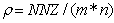 , decreases noticeably for nodes on this 13 level tree from the atom leaves at level 0 to the root node at level 13.• GLPK timing were slightly better than that of
  • LIS timing were slightly worse than
  Note that the binary decomposition strategy is uniquely suitable for very sparse matrix such that only neighboring variables are strongly connected with very little joint rows or columns for variables that are remotely related. CAASD aA applications clearly demonstrate this particular LP-local characteristics. The traditional Bender decomposition with row generation and Dantzig-Wolfe decomposition[3][4] with column generation techniques that do require specific topological structure of the constraint matrix are not directly applicable to Figure 8 as a nesting binary tree.There are challenges that may be overcome later with additional insight and intelligent fine tuning of the key algorithms to resolve outstanding questions regarding its applicability to integer programming, binary programming, parallel computing enhancements, and the ultimate resolution of the worst case computation complexity for the entire class of NPC problems[10].
 | Figure 9. Preliminary LIS Timing Profile With aA Applications |
11. Conclusions and Future Work
In conclusion, the authors present innovative concepts in dealing with very large system of linear inequalities with number of variables and/or constraints close to or over millions. First, all linear systems (equalities and inequalities included) are converted to its homogenous form such that the right hand size are all zeros. This is accomplished by increasing the number of column of the constraint matrix by one and replacing the solution vector, xby twhere  . With linear systems in homogeneous form, linear inequality or equality problems become a searching for a column vector, t, with a constraint matrix, S, such that
 . Consequently, the vector, f, is a measurement of linear feasibility of the solution vector t with respect to the constraints vectors as rows in S. We also demonstrate that if a homogeneous linear inequality system,
  does have a solution with a given initial
  , i.e., not all
  , then one must be able to reduce either the sum of infeasibility computed as the sum of all negative components of the feasibility vector,
  , or the worst case infeasibility as the minimum component of
  (< 0), or the number of rows in S with such a worst case infeasibility. With such insights, we designed three key algorithms aiming to reduce the sum, the worst case, or the number of rows in S with the worst case infeasibility to recursively move from any initial vector,
  to a feasible solution such that
 . Such three key algorithms are a Simplex alike algorithm aiming to reduce the worst case infeasibility in f, a zero-crossing algorithm aiming to reduce the sum of all infeasible rows in S (as revealed by the column vector f=St), and a row de-grouping algorithm that is capable of separating linearly dependent rows in S such that all the rows in S with the worst case infeasibility arelinearly independent. Combining this set of three key algorithms, it is demonstrated that with a computational complexity slightly worse thenthe total number of nonzero elements in the constraints matrix, S, one can locate a solution for the given linear inequality system. This is verified with linear programs (LPs) in self-dual form such that both the prime and the dual systems are explicitly included and a solution exists. These three new algorithms were coded and tested in Java code with the CAASD aviation application, aA, that handles number of variables and/or constraints over one million in a large number of test cases. Experimental test data does show that the answers obtained by such a CAASD Linear Inequalities Solver (LIS), matched exactly solutions obtained from either the Cplex by ILOG, or that obtained with GLPK as the Gnu LP Solver. A preliminary comparison of the CPU time with increasing size in number of variables and constraints are provided. In most cases, the advantage of numerical stability, CPU time vs. problem size, and scalability as described by this paper are demonstrated. Note that such an approach is also applicable to system of linear equalities and Eigen vectors solutions.Major findings of this research are; first, the Simplex alike approach is more economical than the original Simplex as it only applies to rows in S with the worst case infeasibility (minimum value
  of the feasibility vector,
  ); hence, it is much faster and more productive in reducing the worst case infeasibility; second, zero-crossing provides a great number of linear paths to reduce the sum of total infeasibility; and third, row de-grouping is the most efficient way to identify linearly independent rows for the group of rows in S with identical worst case infeasibility for a given column vector, t; fourth, homogeneous liner systems may be scaled to either speed up or increase the precision desired for such an innovative LIS approach; lastly, at high precision, row infeasibility and rounding errors becomes indistinguishable and algorithms can be properly terminated.Note that linear systems in homogeneous form with both equalities and inequalities included does remove the distinction between equalities and inequalities, hence, LIS can be used to solve system of linear equalities just as it solves linear inequalities as
  becomes
 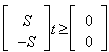 . Namely,
 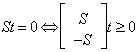 .Furthermore, homogeneous linear systems (equalities and inequalities included) provide a handy normalization process such that rows of the matrix S are all unit vectors and the normalized solution,
  is also a unit vector.Note that unit vectors are numerical stable free from numerical overflow or ill-conditioned problems.Future works include a generalization of the Gaussian Elimination (GGE) for linear systems (equalities and inequalities included) to identify the feasible interval (null, unique, or a real interval with an upper bound and a lower bound). Another piece of our innovative idea for the homogeneous linear systems is to locate a solution or solutions of a homogeneous linear system on the surface of an n-dimensional hyper unit sphere with a radius of 1.0 known as the unit shell (US) with linear subspace projection and the concepts of equal distanced points on the unit shell. Such new ideas are currently under testing by the authors using the Excel tool and java code over very large linear systems with both equalities and inequalities included. The validity of such new innovative ideas is still being pursued and verified. Details of such innovative approaches closely related to the homogeneous linear systems solvers are beyond the scope of this paper. Hopefully, draft papers will soon be available for peer review shortly in additional to this paper on LIS.
ACKNOWLEDGMENTS
The authors acknowledge the helpful review, correction, and editorial advice applied to this draft paper by many of colleagues at MITRE, in particular, Dr. Glenn Roberts,David Hamrick,Dr. Leone Monticone, Dr. Leonard Wojcik, Matt Olson, and Jon Drexler. Our thanks also extended to key CAASD IT Resource Center (ITRC) staff provided the resource, tools, and software support in both conventional and parallel computing. Valuable advice and feedback from SAP reviewers and editors are also greatly appreciated.
References
| [1] | Strang, Gilbert, “Introduction to Applied Mathematics”, John Wiley & Sons Inc., New York, 1979. |
| [2] | Strang, Gilbert, “Karmarkar’s algorithm and its place in applied mathematics”, The Msthematical Intelligencer 9(2): pp. 4-10, New York: Springer, 1987. |
| [3] | Dantzig, G. G. “Maximization of a linear function of variables subject to linear inequalities”, 1947, Published pp. 339-347, in T.C. Koopmans (ed.): Activity Analysis of Production and Allocation, Wiley & Chapman-Hall, New York-London, 1951. |
| [4] | Dantzig, G. B. “Linear Programming andExtensions”.Princeton, NJ: Princeton University Press, 1963. |
| [5] | Fukuda, Komei and Terlaky, Tamas, “Crisis-cross methods: A fresh view on pivot algorithms”, Mathematical Programming: Series B, No. 79, Papers from 16th International Symposium on Mathematical Programming, Lausanne, 1997. |
| [6] | Khachiyan, L. G.,“Polynomial algorithms in linear programming”, U.S.S.R., Computational Mathematical and Mathematical Physics 20 (1980) pp. 53-72. |
| [7] | Karmarkar, N.,“A New Polynomial Time Algorithm for Linear Programming”, AT&T Bell Laboratories, Murray Hill, New Jersey, September, 1984. |
| [8] | Gondzio, Jackek and Terlaky, Tamas, “ A computational view of interior point method”, Advances in linear and integer programming, Oxford Lecture Series in Mathematics and its Applications, 4, New York, Oxford University Press. pp. 103-144, MR1438311, 1996. |
| [9] | Nocedal, Jorge and Wright, Stephen J, : “Numerical Optimization” , Springer Science-Business Media, Inc., 1999 |
| [10] | Michael. R. Garey and David. S. Johnson, COMPUTERS AND INTRACTABILITY, A Guide to the Theory of NP-Completeness, Bell Laboratories, Murray Hill, New Jersey, 1979. |
| [11] | Nemirovsky, A. and Yudin, N. “Interior-Point Polynomial Methods in Convex Programming”, Philadelphia, PA: SIAM, 1994. |
| [12] | Alexander Schrijver, “Theory of Linear and Integer Programming”, Department of Econometrics”, Tilburg University, A Wiley Interscience Publication, New York, 1979 |
| [13] | Niedringhaus, W., “Stream Option Manager (SOM): Automated Integration of Aircraft Separation, Merging, Stream Management, and Other Air Traffic Control Problems”, IEEE Transactions Systems. Man & Cybernetics, Vol. 25 No. 9, Sept. 1995. |
| [14] | Niedringhaus, W., “Maneuver Option Manager (MOM): Automated Simplification of Complex Air Traffic Control Problems”, IEEE Transactions Systems. Man & Cybernetics, May 1992. |
| [15] | Wang, Paul T. R., “Solving Linear Programming Problems in Self-dual Form with the Principle of Minmax”, MITRE MP-89W00023, The MITRE Corporation, July, 1989. |
| [16] | EE236-A, Lecture 15,” Self-dual formulations”, University of California, Department of Electrical Engineering, 2007-08, http://www.ee.ucla.edu/ee236a/lectures/hsd.pdf |
| [17] | ILOG, “Introduction to ILOG CPLEX”, 2007,http://www.ilog.com/products/optimization/qa.cfm?presentation=3 |
| [18] | ILOG, “CPLEX Barrier Optimizer”, 2008,http://www.ilog.com/products/cplex/product/barrier.cfm |
| [19] | Steven Skiena, “LP_SOLVE: Linear Programming Code”, Stony Brook University, Dept. of Computer Science”, 2008 http://www.cs.sunysb.edu/~algorith/implement/lpsolve/implement.shtml |
 Abstract
 Reference
 Full-Text PDF
 Full-text HTML