-
Paper Information
- Paper Submission
-
Journal Information
- About This Journal
- Editorial Board
- Current Issue
- Archive
- Author Guidelines
- Contact Us
American Journal of Computational and Applied Mathematics
p-ISSN: 2165-8935 e-ISSN: 2165-8943
2013; 3(3): 186-194
doi:10.5923/j.ajcam.20130303.06
Second Degree Chance Constraints with Lognormal Random Variables – An Application to Fisher’s Discriminant Function for Separation of Populations
 Abstract
 Reference
 Full-Text PDF
 Full-text HTML
Vaskar Sarkar1, Kripasindhu Chaudhuri2, Rathindra Nath Mukherjee3
1Department of Mathematics, Aryabhatta Institute of Engineering and Management Durgapur, Panagarh, Dist.- Burdwan, Pin - 713148, West Bengal, India
2Department of Mathematics, Jadavpur University, Jadavpur, Kolkata, 700032, West Bengal, India
3Department of Mathematics, Burdwan University, Burdwan, West Bengal, India
Correspondence to: Vaskar Sarkar, Department of Mathematics, Aryabhatta Institute of Engineering and Management Durgapur, Panagarh, Dist.- Burdwan, Pin - 713148, West Bengal, India.
| Email: |  |
Copyright © 2012 Scientific & Academic Publishing. All Rights Reserved.
In this paper, we have discussed a transformation procedure of the second-degree chance constraints to the deterministic constraints for mathematical programming problems having general second degree chance constraints with lognormal random variables. We have used geometric inequality for this transformation. The transformed deterministic problem having non-linear constraints and linear or non-linear objective function can be solved using non-linear programming algorithm. Also we have applied this model to Fisher’s discriminant function for separation of populations. A numerical simulation have been considered along with a graphical representation of the reduced solution region.
Keywords: Stochastic Programming, Chance Constraint Programming, Lognormal Random Variable, Geometric Inequality, Deterministic Reduction, Non-linear Programming, Discriminant Function and Separation of Population
Cite this paper: Vaskar Sarkar, Kripasindhu Chaudhuri, Rathindra Nath Mukherjee, Second Degree Chance Constraints with Lognormal Random Variables – An Application to Fisher’s Discriminant Function for Separation of Populations, American Journal of Computational and Applied Mathematics , Vol. 3 No. 3, 2013, pp. 186-194. doi: 10.5923/j.ajcam.20130303.06.
Article Outline
1. Introduction
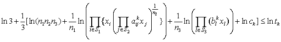
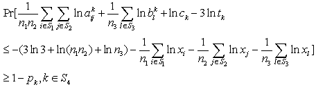
- Stochastic or probabilistic programming[13] deals with the situations where some or all the parameters of the mathematical programming problem are described by stochastic or random variables rather than by deterministic ones. Several models have been presented in the field of stochastic programming[21]. Two major approaches to stochastic programming[13,14] are recognized as:1. Chance constrained programming2. Two-stage programmingThe chance constrained programming (CCP) can be used to solve problems involving chance constraints, i.e., constraints having finite probability of being violated. Its main feature is that the resulting decision ensures the probability of satisfying the constraints, i.e. the confidence level of being feasible. Thus, using CCP, the relationship between profitability and reliability can be quantified. The use of probabilistic constraints was initially introduced by Charnes et al.[6,7], while an early use of probabilistic programming in environmental economics is by Maler[17]. Since then, a number of environmental management case studies use probabilistic constraints[5,10,11,19,22,23]. Also the CCP, in recent years, has been generalized in several directions and has various applications[21].Many authors studied and developed this problem for the parameters having normal distribution, uniform distribution and exponential distribution, where the chance constraints are linear[3, 4, 21]. But lognormal distribution (with two parameters) has a significant role in human and ecological risk assessment for many reasons, of which the main three reasons are (i) many physical, chemical, biological, toxicological and statistical processes tend to create random variables that follow lognormal distributions[12], (ii) lognormal distributions are self-replicating under multiplication and division, i.e. products and quotients of lognormal random variables themselves follow lognormal distributions[1, 9] and (iii) when the conditions of the Central Limit Theorem hold[16], the mathematical process of multiplying a series of random variables will produce a new random variable (the product), which tends (in limit) to be lognormal in character, regardless of the distribution from which the input variables arise[2].Also we may consider the fact that many environmental variables are non-negative means that they are generated by a skewed distribution. Several skewed probability models have been used to describe environmental data, including the Poisson, negative binomial, Weibull, gamma, exponential and the lognormal. Among these distributions, the lognormal has been the most widely applied[18]. In the year 1996, Cooper et.al.[8] noted the importance of using skewed distributions, to represent environmental variables within mathematical programming and lognormal distribution was one among those skewed distributions.So here in our model, we have considered that the parameters of the chance constraints follow lognormal distribution having known mean and standard deviation. In this paper, we have tried to reduce the general second degree (with respect to decision variables) chance constraints to non-linear deterministic constraints, but the objective function, in both of the considered and transformed models, may be linear or nonlinear with deterministic parameters and also we have applied this model to Fisher’s discriminant function for separation of populations[20].
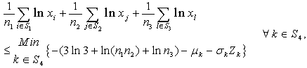
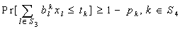
2. Chance Constrained Programming
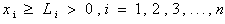
- The chance constrained programming (CCP) involves constraints expressed in terms of probabilities. Chance constrained programming represents risk in a qualitative way, i.e., in chance constrained programming, only the possibility of infeasibility is at stake regardless of the amount by which the constraints are violated. The simplest form of a chance constraint can be given as,
 where,
  is an
is an  matrix usually termed to as a technology matrix,
  is an n-component vector of decision variables,
  is an n-component vector and
  are scalars and the scalar
  stands for the probability with which constraint
  must be satisfied. The scalar
  represents the reliability of decision
  gives the risk of infeasibility associated with decision
 The choice of
  is at the discretion of the decision-maker (DM), in other words, it is a policy maker’s choice, which can be interpreted as an expression of the regulator’s aversion to uncertainty[15]. In this paper we consider that
  and
and  and
and  are independent lognormal random variables with known mean and standard deviation (s.d.).
3. Deterministic Reduction of the Mathematical Model
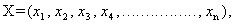
- The generalized form of the second degree chanced constrained programming problem can be written as follows:To find
 so as to,
 | (1) |
 | (2) |
 | (3) |
 and
and  are index sets and
  Here
Here  are all independent lognormal random variables. Let us consider
  ,
,  and also consider that
  are independent lognormal random variables
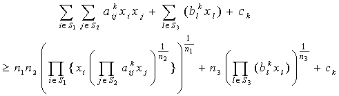
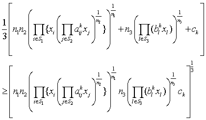
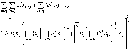
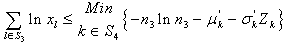
  Here our target is to transform the probabilistic second-degree constraints (2) in to deterministic constraints. We use Geometric Inequality (GI) i.e. AM GM to reduce the constraints in (2) in the following way:We have
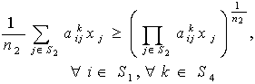 i.e.,
i.e.,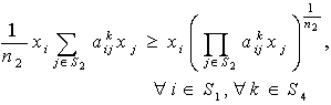 i.e.,
i.e.,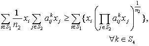 i.e.,
i.e.,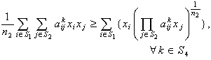 | (4) |
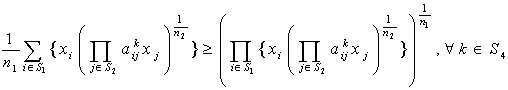 | (5) |
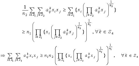 | (6) |
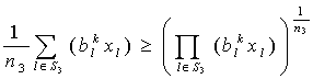 | (7) |
 | (8) |
 | (9) |
 | (10) |
 | (11) |
 i.e.,
i.e., 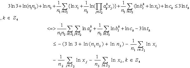 | (12) |
 | (13) |
 are independent lognormal random variables having known mean and standard deviation (s.d.), so
 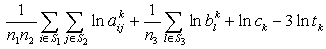 is a random variable having normal distribution with known mean and s.d., say
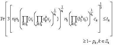
  Thus we have the reduced form of the chance constraints as follows
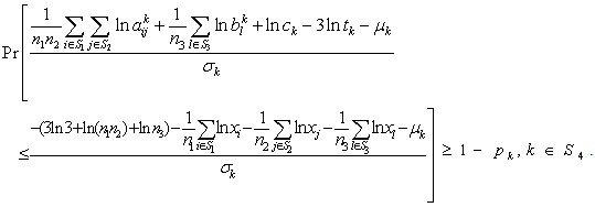 | (14) |
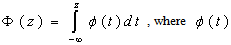 be the probability density function of standard normal variate then we can write,
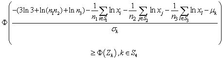 where,
 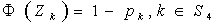 i.e.
i.e. 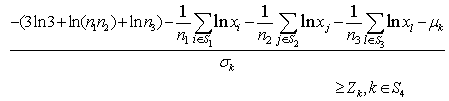 i.e.
i.e. 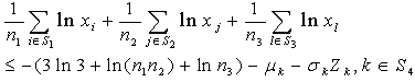 | (15) |
 so as to,
 | (16) |
 | (17) |
 | (18) |
4. Model – A: Model Having Only Second-degree terms in the Chance Constraints
- In this case the form of the chance constrained model, obtained from (1), (2) & (3), is as follows: To find
 so as to,
 | (19) |
 | (20) |
 | (21) |
 are index sets and all
  follows Log-normal distribution with known mean & s.d..So there is no existence of the index set
  Thus the deterministic reduction, having non-linear constraint, of the above model can be obtained from (16), (17) & (18) by just omitting the terms involving
  and the term
 which is as follows:To find
 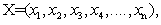 so as to,
 | (22) |
 | (23) |
 | (24) |
 are the mean and s.d. of the normal random variable
 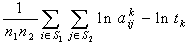 and
and 
5. Model – B: Model Having Only Linear Terms in the Chance Constraints
- Here the form of the chance constrained model, obtained from (1), (2) & (3), is as follows: To find
 so as to,
 | (25) |
 | (26) |
 | (27) |
 is index set.So there is no existence of the index sets
  Thus the deterministic reduction, having linear constraint, of the above model can be obtained from (25), (26) & (27) by just omitting the terms involving
  and the term
 which is as follows:To find
 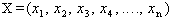 so as to,
 | (28) |
 | (29) |
 | (30) |
 are the mean and s.d. of the normal random variable
 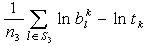 and
and 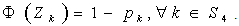 We can rewrite the above deterministic reduction as follows:To find
  so as to,
 | (31) |
 | (32) |
 | (33) |
 are the mean and s.d. of the normal random variable
  and
and 
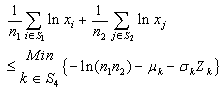
6. Application of the Model in Fisher’s Discriminant Analysis function – Separation of Population
- Fisher derived the linear classification statistic (Johnson and Wichern (2001)) using the following idea:His idea was to transform the multivariate observations X to univariate observations y such that the y’s derived from population
 were separated as much as possible.Fisher suggested to take linear combination of X to create y’s, because they are simple enough functions of the component of X. Also Fisher’s approach does not assume that the populations are Normal and it assumes that the population covariance matrices are equal.So the objective is to select the linear combination of X to achieve the maximum separation of the population mean vectors
  i.e.
i.e. 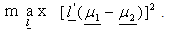 But this does not admit finite solution for
  To make the problem meaningful, Fisher considered the standardized ratio
 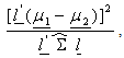 that is, to find
  so as to
 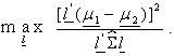 This admits finite solution for
  Alternatively, one may write the above problem, in case as follows
  is unknown and can be estimated by
  and
and  are known, as follows: To find
  so as to
 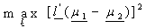 subject to,
 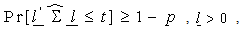 where p (> 0) be very small.Here, let us consider that,
  component-wise follows lognormal distribution with known mean and s.d. where
 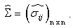 So the above problem reduces to the following form:To find
  so as to
  subject to,
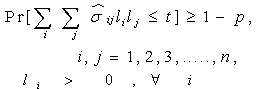 where,
  Here
Here  follows lognormal distribution for all i,j ,with known mean and s.d. and t ( > 0 ) is some suitable constant (very small). Then using Model – A, the above problem can be solved.
 7. Managerial Application
- Waste water pollution can be controlled, at the river and associated land, either by emission restrictions of waste water or by land and water use restrictions. Typically the direct control of emissions is impossible due to the high cost of observing industry emissions. A further problem is that waste water emissions, which are determined by production events of industries, are stochastic and this leads to wide variations in the waste water pollution concentrations in surface and groundwater. Thus in practice the regulatory body is unable to apply deterministic water quality standards, but instead, must set reliability level which states that the minimum standard must be met for some proportion of the time. In setting this reliability level the regulatory body trades off reliability against associated costs. Also in the study of waste water pollution control, we focus our attention to probabilistic programming, because in most of the environmental management problems, quantitative data on the cost of exceeding emission standards are impossible to estimate. This is the case with waste water emissions where the costs of exceeding the standard would include health costs and a range of costs due to ecological damage. Our models can be used suitably to such problems based on relevant data collected through field work.
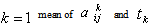
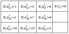
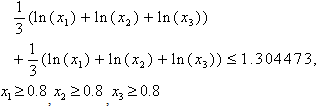
8. Numerical Example
- Let us consider the following maximization problem:To find
 so as to
 | (34) |
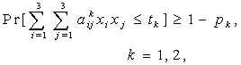 | (35) |
 | (36) |
 follows independent lognormal distribution with known mean & s.d. and
|
|
|
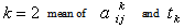
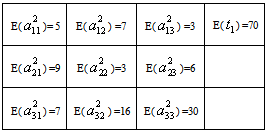
|
 subject to,
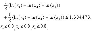 The global solution obtained using optimization software ‘Mathematica 5.2’ is as follows:
 Also using generic package ‘MATLAB 7’ we have verified that, this solution satisfies the constraints (35). Thus the optimal solution to the given problem is as obtained above.
9. Discussion
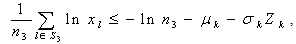
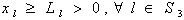
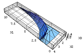
- In this paper, we have reduced the probabilistic constraints to deterministic constraints. The reduced deterministic constraints along with the feasibility conditions i.e.,
 generates the solution region as shown in the following figures.
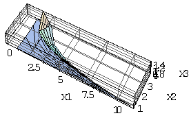 | Figure 1. Reduced solution region |
 | Figure 2. Different angle view of reduced solution region |
10. Conclusions
- The basic objective of this work is to reduce the probabilistic constraints to deterministic constraints through implicative relationship. While reducing the probabilistic constraints to deterministic constraints, the event space under consideration has been enlarged. As a result, implicative reduction calls for verification of whether the optimal solution under extended region satisfies the original chance constraints or not. Once this verification gives a positive response, the obtained optimal solution of the extended problem becomes the optimal solution of the original problem. In case of a tight extension of the original problem, the positive response during verification becomes a likely one. Indirectly, tight reduction through implicative relationship calls for use of sharp inequalities including separation of coefficient parameters, if needed under distributional assumption. For a lognormal setup, separation of coefficients from the lognormal variables is a must, because often wise evaluation of the resultant distribution becomes a tedious task. For a normal setup, this separation is redundant. Moreover for some distribution the joint probability distribution for large number of random variable can be evaluated using mathematical induction method[3]. But for some distribution, like lognormal, it is often become impossible to find joint probability distribution for large number of random variable. In that case our method is very much useful to reduce the probabilistic constraints to deterministic one. Further, more refinement of the solution may be possible applying the concept of genetic algorithm to the present solution.