H. P. Rani1, T. Divya1, R. R. Sahaya2, Vivekanand Kain3, D. K. Barua2
1Department of Mathematics, NIT Warangal, Warangal, 506004, India
2Nuclear Power Corporation of India Limited, BARC, Mumbai, 400 085, India
3Corrosion Science Section at Materials Science Division, BARC, Mumbai, 400 085, India
Correspondence to: H. P. Rani, Department of Mathematics, NIT Warangal, Warangal, 506004, India.
| Email: |  |
Copyright © 2012 Scientific & Academic Publishing. All Rights Reserved.
Abstract
This paper describes the turbulent flow of water through the orifice and double elbow using the Reynolds stress turbulence model. The characteristics of turbulent flow near the solid wall have been examined. The turbulent parameters such as velocity, kinetic energy and Reynolds stresses are analyzed in terms of the non-dimensional wall distance parameter y+ values (0 < y+ < 650) for three different Reynolds numbers (Re) at the critical location of the corresponding components. These simulated results are validated with the literature results for each component, and are found to be in good agreement. In general, for high Re number, inertia forces dominated over viscous forces. It is observed from this analysis is that these inertial forces and other parameters attained their peak values in the log law layer (30 < y+ < 500) or in the outer layer (y+ > 50), whereas the minimum values of these parameters are observed in the viscous sub layer (y+ < 5) or in the viscous wall region (y+ < 50).
Keywords:
Turbulent, Orifice, Double Elbow, y+
Cite this paper: H. P. Rani, T. Divya, R. R. Sahaya, Vivekanand Kain, D. K. Barua, Turbulent Flow in the Vicinity of Solid Walls in an Orifice and Double Elbow, American Journal of Computational and Applied Mathematics , Vol. 3 No. 3, 2013, pp. 174-181. doi: 10.5923/j.ajcam.20130303.04.
1. Introduction
The study of turbulent flow parameters near the solid surface of pipes has importance in various engineering disciplines and attracted many investigations. The orifice pipe and double elbow are most commonly used components in the piping system of many industries[1, 2]. For the safety of piping systems it is mandatory to analyze the flow, and the parameters which are leading to failure in these components. Failures have occurred in the components in which the recirculation regions exist, such as sudden expansion, orifice, elbows etc.[3]. The measurements of turbulent parameters in terms of non-dimensional wall distance greatly assisted in correlating the experimental data[4]. The present study is about the investigation of turbulent parameters in terms of non - dimensional wall distanceparameter, y+, in the orifice and double elbow. The downstream of the critical locations in the orifice and elbows are given prior importance in this study, since these are more critical regions susceptible to failures[3, 5]. Specifically, the region at the downstream of the orifice and the region at the downstream of the second elbow in the double elbow with 30 < y+ < 500 are mainly of concern. This study has been carried out for the three different Reynolds numbers (Re) values: 2e+4, 4e+4 and 6e+4. The turbulent parameters such as velocity, Reynolds stresses along with the turbulent kinetic energy are calculated in the region of interest. The behavior of these parameters in the various wall regions and layers in terms of y+ was investigated. In section 2, a detailed geometrical description about the proposed orifice and double elbow models are explained along with the governing equations, such as, mass,momentum, turbulence, energy and species transportation of the incompressible fluid flow. In section 3, the grid generation and the numerical methods for solving the above governing equations are discussed. In section 4, the validation of the present results is shown. All the turbulent parameters in terms of y+ values with respect to Re are plotted and analyzed. Finally, the conclusions are given in section 5.
2. The Problem Description and Governing Equations
In the present study two-dimensional, turbulent, steady and fully developed flow of water reaching the orifice and double elbow geometries with diameter (D) 0.0254m[1, 2] is considered. The geometry of physical problem considered in this study along with the coordinate system used is shown in Fig.1. The tube with a circular orifice is assumed to be of length 9D and is of height D as shown in Fig. 1(i). This orifice is assumed to be of thickness 0.0032m (B) and of diameter D/2. The angle of the bend is assumed to be 90o in the double elbow pipe (Fig. 1(ii)), and the pipe is of length 23D with a total height of 4D. The upstream and downstream lengths of critical locations such as flow singularity locations were chosen to be large. These considered lengths reduced the effect of inlet and outlet boundary conditions on the flow patterns in the vicinity of the wall. At the flow singularity locations, these patterns are consistent with other studies in the literature and this validation is shown in section 4.1.The governing equations, along with the boundary and flow conditions and the method of solution applied to model the turbulent flow of water in the considered geometries are described below.Governing equationsThe flow is governed by the basic equations such as the conservation of mass, momentum and energy together with the species transport. Also to model the turbulent flow, the equations of turbulent kinetic energy (TKE), and its dissipation rate (DR), are considered. The flow is considered as steady, thus, the temporal terms have been eliminated. The fluid is assumed to be incompressible; hence the changes in the density are neglected. To illustrate the influence of turbulent fluctuations on the mean flow, the flow variable  is considered to be the sum of mean velocity
  and fluctuating velocity
  Then, the resultant equation for the conservation of mass is given by
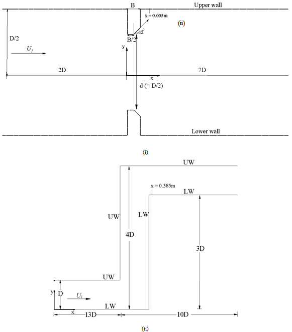 | Figure 1. Computational geometries of the present study, with the diameter D = 0.0254m, the orifice thickness B = 0.0032m, UW is upper wall, LW is lower wall and x is the axial location at which Figs. 3-6 are drawn |
 | (1) |
The Reynolds time averaging equation for momentum is given by | (2) |
where ρ is the density, p is the static pressure, ν is the kinematic viscosity of the fluid and  is the turbulent shear stress or Reynolds stress. The convention of thisnotation is that i or j = 1 corresponds to the x-direction, i or j = 2 for the y-direction. By using the Boussinesq theorem,
  in Eq. (2) is proportional to the average velocity gradient, and can be calculated as
  | (3) |
where  is the turbulent kinematic viscosity. This viscosity was calculated using Reynolds stress model[4] and this model is discussed in the next subsection. Equations (1) and (2) were solved along with the following energy equation:
 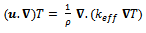 | (4) |
where, T denotes the temperature, 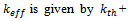
 with turbulent Prandtl number Prt = 0.85, kth denotes the thermal conductivity,
  is the specific heat at constant pressure and
  is the turbulent eddy viscosity.The conservation equation of the chemical species, which predicts the local mass fraction of species (ferrous ions), takes the following general form:
 | (5) |
where the mass diffusion flux of species is defined as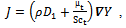 with constant turbulent Schmidt number (Sct = 0.7); Y is the local mass fraction of the species and D1 is the diffusion coefficient of the species.To compute the turbulent kinematic viscosity, νt given in eq. (3), several turbulence closures and near-wall treatments are available in the Fluent CFD 12.1 software code ranging from k-ɛ type models to full Reynolds stress models[6]. The Reynolds stress turbulence model[4] is employed to predict the Reynolds stresses along with the TKE (k) and DR (ε). The turbulent kinematic viscosity,
  given in Eq. (3), was computed by combining k and ε as
  | (6) |
where Cµ = 0.09.Reynolds Stress ModelThe eddy-viscosity approximation ignores the effect of upstream history upon the Reynolds shear stress. Durbin[7] mentioned that, by carrying a differential equation for the Reynolds shear stress we can obtain considerably better results for the adverse-pressure-gradient boundary layer with large pressure rise. The most complex classical turbulence model is the Reynolds stress equation model, also called as the second-order or second moment closure model. The prediction of flows with complex strain fields or significant body forces leads to several major drawbacks by using the k-ε model. In these conditions the individual Reynolds stresses are poorly represented by the following Boussinesq relationship even if the TKE is computed to reasonable accuracy. 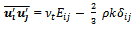 | (7) |
where and Kronecker delta i.e.,
 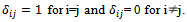 The exact Reynolds stress transport equation on the other hand can account for the directional effects of the following Reynolds stress field equation[4]:
 | (8) |
where the Reynolds stress  The above eq. (8) describes three partial differential equations: one for the transport of each of the three independent Reynolds stresses and these terms are expressed in the following equations (9) - (12):The production term
 in its exact form is
 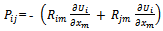 | (9) |
The diffusion term ( ) can be modelled by the assumption that the rate of transport of Reynolds stresses by diffusion is proportional to the gradients of Reynolds stresses as
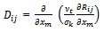 | (10) |
with  The dissipation
  is modeled by assuming isotropy of the model small dissipative eddies as
 | (11) |
The transport of  due to turbulent pressure strain interactions
  is given by
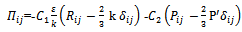 | (12) |
with 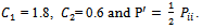 Turbulent kinetic energy (k) is needed in the above formulae and can be found by adding the three normal stresses together i.e.
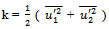 | (13) |
The six equations for Reynolds stress transport are solved along with a model equation for the scalar dissipation rate ε. Again a more exact form is found by Launder et al.[8], but the following equation from the standard k-ε model is used in commercial CFD softwares for the sake of simplicity. 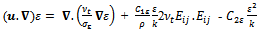 | (14) |
where the adjustable model constants have the default values as C1ε=1.44, C2ε =1.92 and the Prandtl number of ε is 
3. The Generated Mesh and the Computational Procedure
The equations (1) - (5) which govern the two-dimensional pipe flow are analyzed using the well-developed commercially available software, namely, ANSYS. In the first analysis phase, the geometry of the flow model is constructed using the grid-generation software, namely, ANSYS Workbench. The non-uniform grids are generated and clustered in the vicinity of bounding walls. While generating this mesh, the distance between the first calculating node and the wall is chosen to be so small to have the distance from the wall measured in viscous lengths, < 500. First cell height = R.F.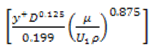 | (15) |
where the R.F. is refinement factor and it was considered to be one to create the fine mesh[6].The flow volume, boundary and initial conditions for this model have been provided in the ANSYS FLUENT 12.1[6]. In the present study, some of the boundary conditions for the pipe failure conditions applied by Pietralik and Schefski[5] are considered. The uniform velocity is used as the inlet boundary condition. The boundary conditions imposed on the wall are no-slip for momentum, constant temperature for thermal and constant concentration for species. At the outlet, the zero-gradient properties are considered to be linear for the pressure. The critical temperature is considered as 310℃[5], the constant wall roughness as 7.5e-5 m[5], the Schmidt number, as 9.2[5], the Prandtl number,
  as 8.911. The moderate
  values 2e+4, 4e+4 and 6e+4[10] are considered to analyze the flow.The SIMPLE algorithm is used along with the staggered grid to simultaneously solve the velocity and pressureequations. The second order upwind scheme was used fordiscretising the convection and diffusion transports on a uniform grid. In all the investigations, the iterative calculations of the primitive variables, such as u, k, ε, T and Y were terminated when the residual norm criteria of 1e-6 are reached. In the final stage, the predicted results were viewed and analyzed by the animated plotting tool, namely, FLUENT postprocessing. The computations were carried out using the work station HP Z800 Intel Xeon Dual Core Processor.
4. Results and Discussion
We begin by presenting the numerical validation of the present study in the orifice and double elbow with previous results of Smith et al.[1] and Debnath et al.[2], respectively. Then, the distribution of turbulent parameters at the critical location of the corresponding component have beeninvestigated in terms of following wall spacing parameter (ΔS) for different y+ values(0 < y+ < 650) and for different Re, | (16) |
where uf is the friction velocity, 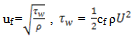 and cf is given by Schlichting skin-friction correlation[9] as
 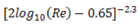 for Re < 109.As wall spacing values (ΔS) is a function of y+ and Re, the dependency of these variables are analyzed in detail. From equation (16) it can be noted that the calculated ΔS values differ corresponding to the y+ values (0 < y+ < 650) for fixed Re. Also the range of ΔS for 0 < y+ < 650 varies for different Re values. Also the grid independency test has been carried out for three different grid sizes and the details are tabulated in Table 1. For the present study the grid size in bold face in Table 1 are selected for the simulation.
Table 1. Grid Independence test
 |
| |
|
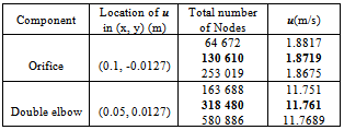
It is observed that the different sizes of recirculation zones reside near the bend zones of the elbow. From Fig. 2, it can be noted that, the present simulation results are in close agreement with the published numerical results in the literature.
4.1. Turbulent Parameters
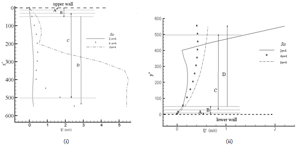
As the considered Re values are high, the viscous stresses are negligible everywhere in the computational region and small compared with the Reynolds stresses. Hence in the present study the turbulent parameters such as velocity,Reynolds stresses and kinetic energy are examined at the critical location of each component for different Re values in terms of y+ values. The critical locations in the orifice and double elbow were selected by the deep analysis of failures in these components as discussed by Ahmed et al.[3] and Pietralik and Schefski[5], respectively. At these critical locations the turbulent parameters are analyzed since these parameters will play a vital role to study the failure analysis[3, 10]. The study of these parameters is examined in terms of y+, since this parameter greatly assisted in correlating theexperimental data[4]. The different layers are defined based on the y+ values such as viscous sub-layer (y+ < 5), viscous wall region (y+ < 50), log – law layer (30 < y+ < 500) and outer layer (y+ > 50) are denoted as A, B, C and D, respectively in Figs. 3-6. The values in the orifice at x = 0.005m from the upper wall is shown in (i) and the values in the double elbow at x = 0.385m from the lower wall for 0 < y+ < 650 are shown in Figs. 3-6 (i) and (ii), respectively. | Figure 2. Comparison of simulated results with the previous results |
 | Figure 3. Velocity magnitude in the (i) orifice at x = 0.005m (shown in Fig. 1(i)) from the upper wall (ii) double elbow at x = 0.385m (shown in Fig. 1(ii)) from the lower wall. A, B, C and D denotes the viscous sub layer (y+ < 5), viscous wall region (y+ < 50), log-law layer (30 < y+ < 500) and outer layer (y+ > 50), respectively. In the next Figs. 4 - 6 same notations are used for A-D and x |
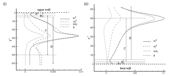 | Figure 4. For Re = 2e+4 the simulated Reynolds stresses (ui2, uj2and uiuj) along with kinetic energy (k) (i) orifice at x = 0.005m from the upper wall (ii) double elbow at x = 0.385m from the lower wall. The other notations are same as in Fig. 3 |
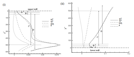 | Figure 5. For Re = 4e+4 the simulated Reynolds stresses (ui2, uj2and uiuj) along with kinetic energy (k) (i) orifice at x = 0.005m from the upper wall (ii) double elbow at x = 0.385m from the lower wall. The other notations are same as in Fig. 3 |
 | Figure 6. For Re = 6e+4 the simulated Reynolds stresses (ui2, uj2and uiuj) along with kinetic energy (k) (i) orifice at x = 0.005m from the upper wall (ii) double elbow at x = 0.385m from the lower wall. The other notations are same as in Fig. 3 |
VelocityFigure 3 presents the velocity magnitude for different Re values. In the orifice, it was observed from the Fig. 3(i) that in all the layers the velocity increases with respect to increased Re and the velocity changes rapidly in 30+<500.Also observed that velocity increases drastically with respect to Re in the log-law layer, since the inertial forces always dominate in this region, specifically for high Re[11]. In the double elbow, from Fig. 3(ii) similar observations are noted in the log-law layer with respect to Re. Also, the velocity magnitude increased with the increased Re values till y+ < 400. After that suddenly the velocity increases for Re value of 2e+4 due to the distance ΔS value very near to the center line. Also this velocity value is more than that of other values of Re due to the decrease of wall distance (ΔS) with the increased Re.Reynolds stresses and Kinetic energyFigures 4 – 6 present the Reynolds stresses (ui2, uj2 and uiuj) along with the kinetic energy (k) in different layers and for different Re. For Re = 2e+4 (Fig. 4) in the viscous wall region y+ < 50 (region B) all the parameters in orifice (Fig. 4(i)) and double elbow (Fig. 4(ii)) are decreased, except shear stress in the orifice. After that, all the parameters, including the shear stress, are increasing with respect to y+ value and attain the peak value in the log law layer (region C) at y+= 300 for orifice and at y+= 500 for double elbow and then decreasing in the outer layer (region D). Also observed that Reynolds normal stresses (ui2, uj2) have the higher values along with turbulent kinetic energy (k) in comparison with the shear stress(ui uj). For orifice, the shear stress (uiuj) has the negative values only near the wall region (B), but for the double elbow, shear stress has the negative value through out the region y+ < 450. Similar observations are made for Re = 4e+4 and 6e+4 from Figs. 5 and 6 with some variations with that of Re = 2e+4. Those observations are:• shear stress is also decreasing in the viscous wall region (region B) of orifice (Figs. 5(i) and 6(i)).• shear stress is having the negative values in the entire region (regions A-D) of double elbow (Figs. 5(ii) and 6(ii)) due to the flow reversal at higher flow rates[12]. • the increased Re results in increase of all the parameters, except the shear stress in the double elbow due to the negative stress.• all the parameters attain their peak values in the region away from the wall• from Figs. 4(i) - 6(i), for orifice as Re increases these peak values exist in the log-law region(C) and move to the outer region. From 4(ii) – 6(ii), for the double elbow as Re increases these peak values exists at the end of the log law region and move to the outer region.Thus it can be concluded that Reynolds stresses and turbulent kinetic energy behave differently with respect to y+. In the orifice, shear stress behaviour is different with respect to all other parameters in the viscous wall region, but similar in the log-law layer (C) and outer layer (D) for all the considered Re values. In the double elbow, shear stress behaviour is different with all other parameters in the entire region of 0 < y+ < 650 due to negative shear stress in that region.
5. Conclusions
In the present study the steady, turbulent, two-dimensional flow of water in the two components (the orifice and double elbow) are considered. The characteristics of turbulent flow near the solid wall was examined for three different Reynolds numbers (2e+4, 4e+4 and 6e+4) using the Reynolds stress model. The turbulent parameters such as velocity, kinetic energy and the Reynolds stresses are analysed in terms of the y+ values (0 < y+ < 650) at the critical location of the corresponding components. These simulated results are validated with the reported results from literature for each component, and are found to be in good agreement. It is observed from this analysis that since the considered Re values are high, inertial forces dominates than the viscous forces. Also observed that these inertial forces and other parameters except shear stress in the double elbow are attaining the peak values in the log law layer (30 < y+ < 500) or in the outer layer (y+ > 50), since always the inertial forces dominate in this region especially for the high Re numbers. However, the minimum values of these parameters are observed in the viscous sub layer (y+ < 5) or viscous wall region (y+ < 50). In the orifice, shear stress behaviour differed with all other parameters in the viscous wall region, but showed a similar trend in the log-law layer and in the outer layer for all the considered Re values. In the double elbow, the shear stress behaviour differed with all other parameters in the entire region of 0 < y+ < 650 due to negative shear stress in that region. In both the geometries, the increased Re resulted in increase of all the parameters in the double elbow due to the negative stress.
ACKNOWLEDGEMENTS
The financial support from the Board of Research in Nuclear Sciences, under BRNS/2009/36/70-BRNS/2390,Department of Atomic Energy is gratefully acknowledged.
References
| [1] | Smith, E., Artit, R., Somravysin, P. and Promvonge 2008, Numerical investigation of turbulent flow through a circular orifice, KMITL Science Journal, 8(1), 43-50. |
| [2] | Debnath, R., Somnath B., Arindam M., Roy D., and Snehamoy M., 2010, A comparative study with flow visualization of turbulent fluid flow in an elbow, International journal of engineering science and technology, 2(9), 4108-412. |
| [3] | Gammal, M. Al., Ahmed, W. H.and Ching, C. Y., 2012,Investigation on wall mass transfer characteristics downstream of an orifice, Nuclear Engineering and Design, 242, 353-360. |
| [4] | H. K. Versteeg and Malalasekera W., An Introduction tocomputational fluid dynamics the finite volume method, 1st ed., Longman, 1995. |
| [5] | Pietralik, J. M., and Schefski C.S., 2011, Flow and mass transfer in bends under flow-accelerated corrosion wall thinning conditions, Journal of Engineering for Gas Turbines and Power, 133, 012902-1 - 012902-7. |
| [6] | ANSYS Fluent® version 12.1 Users Guide, 2009. |
| [7] | Durbin, P.A., 1993, A Reynolds stress model for near-wall turbulence, Journal of Fluid Mechanics, 249, 465- 498. |
| [8] | Launder, B. E. and Spalding, D. B., Mathematical Models of Turbulence. Academic, 1972. |
| [9] | Schlichting and Hermann, Boundary Layer Theory, 7th Edition, McGraw-Hill, 1979. |
| [10] | Ahmed, W.H, Bello M.M., Nakla M.N. and A.A. Sarkhi, 2012, Flow and mass transfer downstream of an orifice under flow accelerated corrosion conditions, Nuclear Engineering and Design, 252, 52-67. |
| [11] | Pope, S.B., Turbulent flows, Cambridge University, 2000. |
| [12] | Gijsen F.J.H., F.N. van de Vosse, and Janssen J.D., 1998, Wall shear stress in backward-facing step flow of a red blood cell suspension, Biorheology, 35, 263–279. |
 Abstract
 Reference
 Full-Text PDF
 Full-text HTML