1. Introduction

The Voronoi diagram is often broadly described as the partitioning of the plane containing a set of sites into disjoint regions such that the area enclosed by each region is closest to its internal site (i.e., each region is closest to a single site). This instance of the Voronoi diagram is more known as the 1^st-order Voronoi diagram. The properties and computations of the 1^st-order Voronoi diagram of point sites are very well researched and provide the foundations to generalize the solution in more ways than this paper will cover[1,2]. The focus will be on elementary properties of the 1^st-order Voronoi Diagram and generalization to different geometrical sites and distances.

2. 1^st-Order Voronoi Diagram

Let P be a set of n points in the Euclidean plane. The 1^st-order Voronoi diagram, denoted VD(P), partitions the plane into n disjoint regions such that the area bounded by each region is closest to a single site than any other site . There are a variety of remarkable properties of the edges, vertices, and cells of the Voronoi diagram which will be examined along with a well known algorithm that is used to compute VD(P) known as Fortune’s algorithm.

2.1. Voronoi Edge

Every Voronoi edge is the locus of points that are closest and equidistant to two sites . Let be the Euclidean distance between two sites and . Then the Voronoi edge can be defined by The

equality represents the perpendicular bisector of the line segment while the inequality restricts the Voronoi edge to be only the closest points on the perpendicular bisector. Hence every Voronoi edge is a line, a ray, or a line segment[1].

Since the locus of points equidistant from a point x lie on a circle centered at x, contains the centre of every empty circle passing through both p and q[2].

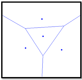Figure 1. Voronoi diagram of 4 point sites. Note that the three Voronoi edges that intersect the border are rays

2.2. Voronoi Vertex

A Voronoi vertex is defined to be the centre of the largest empty circle circumscribing three sites Figure 2 displays the empty circumcircles of the Voronoi vertices. This definition requires that no four sites are co-circular. In the event that four sites are co-circular, two Voronoi Vertices are created, each of degree 3 containing a “zero-edge” between them[1]. Intuitively, n co-circular sites should have a Voronoi vertex of degree n, so the zero-edges are often removed after the initial computation[1].

2.3. Voronoi Cell

The Voronoi cell of a site, denoted is the intersection of half-planes bounded by each for every nearest neighbour. Hence there are exactly n cells. Each cell is convex but not necessarily bounded. In fact, is unbounded if and only if p is on the boundary of the convex hull of P[1].

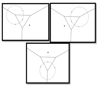Figure 2. Circumcircle for each of the three Voronoi Vertices. Each green point is equidistant to the centre of the given circle

A remarkable feature of the 1^st-order Voronoi Diagram is its locality. That is, if a Voronoi Diagram of a point set is known, then the addition of new sites into the original set results only in a change of the Voronoi cell in which the new site is located, and possibly to its adjacent Voronoi cells.

2.4. Delaunay Triangulation

The dual of the Voronoi diagram is obtained by creating segments between every pair of point sites that share an edge[2]. The result is the Delaunay triangulation of the point set. The Delaunay triangulation has an enormous amount of applications, and in itself exemplifies the usefulness of the Voronoi Diagram. See Figure 3 for an illustration.

Applying Euler’s formula, an upper bound for the number of vertices and edges in the Voronoi Diagram can be derived. However, the Voronoi Diagram contains unbounded cells, so Euler’s formula is not applicable initially, but the dual is necessarily finite, connected and planar. Let n, e, f denote the number of vertices, edges, and faces of the Delaunay triangulation of a set of points P. By Euler’s formula, . Since every edge is incident to two vertices, and every vertex has a degree of 3, the following inequality holds: . By rearranging and substituting the first equation into the above inequality, an upper bound on the number of edges and faces can be derived; hence, the Delaunay triangulation has edges (which dualize to Voronoi edges) and faces (which dualize to at most Voronoi Vertices)[2].

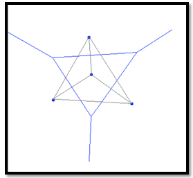Figure 3. Obtaining the Delaunay triangulation from the Voronoi diagram

2.5. Fortune’s Algorithm

There are many algorithms that compute the 1^st-order Voronoi diagram. For instance, the given definition of Voronoi cell immediately suggests that we can compute the Voronoi cell of each site by intersecting half-planes bounded by perpendicular bisectors of segments adjoining two sites. Without using more sophisticated techniques (such as divide-and-conquer) this computation can result in a time complexity of [3].

Fortune’s algorithm uses a sweep line to compute the Voronoi diagram of a point set in time[1]. A vertical (or horizontal) line sweeps the plane and determines when events are encountered and calls upon the necessary event-handler. Three main features characterize the algorithm: the beach line, site events, and circle events.

Recall that the locus of points equidistant to a point p and a line l is a parabola with focus p and directrix l. Now let l be the sweep-line. Upon intersecting a point site, a parabola is created using the definition above. Initially a parabola will have zero-width – it is just a ray perpendicular to l. While the sweep-line proceeds, the parabola becomes wider and will be intersected by other parabolas as more point sites are intersected by l. The intersections of parabolas are called breakpoints and they trace the edges of the Voronoi diagram. The union of these parabolic arcs truncated at breakpoints compose the beach line and is the invariant throughout this algorithm. That is at any given time during the plane sweep, the beach line is equidistant to the line l and some point site(s) in the swept portion of the plane. It is represented by a binary search tree that stores the breakpoints as internal nodes and parabolic arcs as leaf nodes[1].

Site events are detected as the sweep line intersects a new point site. Hence there are exactly n site events. A new arc appears on the beach line only through site events. Furthermore, each new parabolic arc results in the splitting of at most one arc into two. Thus the beach line will consist of at most arcs[1].

Every Voronoi vertex is determined by a circle event[1]. A circle event occurs when the sweep line intersects an empty circle circumscribing three point sites at a single point – hence the circle is fully contained within the swept portion of the plane and will remain empty throughout the remainder of the sweep. This moment of tangency of the empty circumcircle coincides with the elimination of an arc on the beach line. As the sweep line reaches a circle event, two consecutive breakpoints on the beach line converge to a single point, eliminating an arc. The intersection of these breakpoints is the centre of the circumcircle and is a Voronoi vertex by definition[1].

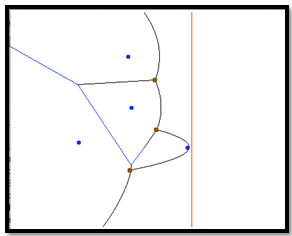Figure 4. Fortune’s algorithm. The red sweep line is the directrix for each parabolic arc on the beach line. Each breakpoint has been highlighted in brown

Figure 5. Circle events are realized and disregarded through site events. Notice at this point during the sweep, there are two possible circle events

On a set of non-collinear point sites, the beach line will contain triples of consecutive arcs[1] as illustrated in Figure 4. Each site event introduces a new parabolic arc to the beach line, which results in the formation of new triples of consecutive arcs and in some cases the elimination of previous triples. Each triple defines a potential circle event, but some of these may be false alarms and will therefore not be handled. Indeed, if a site event results in the new parabola intersecting a triple in its middle arc that triple ceases to exist and moreover, the site is necessarily inside the circumcircle associated with the previously existing triple. It follows that the number of circle events processed corresponds exactly to the number of Voronoi Vertices in the diagram, [1]. Figure 5 shows an instance during the plane sweep where two possible circle events are in the event queue.

If we enclose the set of points in a bounding box, then the infinite Voronoi edges will intersect the edges of the box and therefore the Voronoi diagram can be stored as a finite subdivision in a doubly connected edge list. Because each site defines exactly one Voronoi cell, Fortune’s Algorithm uses storage[1].

3. Generalization of the Sites

Representing physical objects as point sites is appropriate in a lot of different contexts (e.g. industries, institutions, schools over a large geographical area) and is very good for locational analysis. But perhaps the question we are interested in has to do with motion planning, in which case the path that is equidistant to two barriers determines an object’s ability to maneuver around them. Physical objects can be approximated well by polygons and conics. To this end, the Voronoi diagram of line segments and circles will be examined.

3.1. Line Segments

The notion of mid-set changes in regards to the geometrical structure of the sites in the Voronoi diagram. Up until now the mid-set between any two sites was a line segment, a ray, or a line. As sites within this model have endpoints and interiors, we now must consider the locus of points equidistant to a point and a line segment, to two points, and to a point and a line segment. These are obviously a parabola, perpendicular bisector, and angular bisector respectively. If two sites share an endpoint, then their mid-set can have area. This has implications not only in the computation of the Voronoi diagram but it’s storage as well and is avoided by perturbing two site’s common endpoints by a small amount. To this end, the Voronoi diagram of a set of non intersecting, disjoint line segments will be detailed

From the above discussion on mid-sets, it is clear that Voronoi edges are now comprised of line segments, parabolic arcs, and rays. Despite the change in topology, the fundamental nature of these edges remains the same; that is they are locally furthest away from exactly two neighbouring sites. One final important consideration is the locus of points equidistant to a site endpoint and its interior. This is realized by the line through the site’s endpoint that is perpendicular to its interior. Even though this line is not a Voronoi edge (as only one site is involved), it is crucial to the construction of the line segment Voronoi diagram[1].

Fortune’s Algorithm can be refined to handle disjoint line segments. Similar to the case for point-sites, it is required that no four line segments are tangent to a common empty circle. At any moment, the beach line must be equidistant to the sweep line and the closest sites that have already been swept. Hence, the beach line will consist of parabolic arcs and line segments. The breakpoints between arcs and line segments can be classified as one of two types: those associated with two sites and those associated with one[1].

If a breakpoint is equidistant to two sites then it either traces a line segment (i.e. the mid-set of two site endpoints, or two site interiors) or a parabolic arc (i.e. the mid-set of a site endpoint and another site’s interior). In either case, the breakpoints trace a Voronoi edge[1].

The second type of breakpoints trace line segments but are not Voronoi edges as they are equidistant to exactly one site. These breakpoints either trace the mid-set of a site’s endpoint and interior (as discussed above) or is the result of the sweep line intersecting a site’s interior, in which case the breakpoints trace the site’s interior and is incident to the sweep line[1].

Site events occur when the sweep line intersects a site’s endpoints. At an upper endpoint, an arc on the beach line is intersected by a degenerate parabola and is split into two. As the sweep line intersects the site’s interior three breakpoints of the second type split the parabola into 4 arcs (as a result of the distinction between points equidistant from a site and its interior). Finally, when the sweep line reaches the lower endpoint of a site, the breakpoint that traced the sites interior is replaced by two breakpoints (equidistant from the site’s lower endpoint and interior) containing a parabola between them[1].

Circle events are anticipated in the same way they were for point-sites (i.e. the convergence of breakpoints) but come in two forms. Note that the breakpoints that trace a site’s interior are not involved in circle events. If two breakpoints of the first type converge towards a single point then this point is the centre of the empty circle tangent to three sites. However if either of these breakpoints are of the second type then their intersection is the centre of the empty circle tangent to a site at its endpoint. In this case the Voronoi vertex has degree 2 and is incident to a parabolic arc and line segment[1].

Despite the slightly more complicated edges of the Voronoi diagram, it can still be computed in time and can be stored in a doubly connected edge list, using storage[1].

3.2. Circles

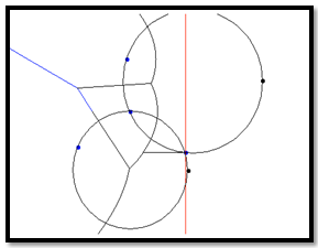
Generalizing the Voronoi diagram to a set of circle sites can be done in the same way it was done for line segments: with careful consideration of the mid-set of the sites. To be thorough, we must consider circles of different radii that are allowed to intersect one another. The locus of points equidistant to two non-intersecting circles is a hyperbola defined by the two centres of the circles as foci with the difference between the distances from the hyperbola to each of the foci equal to the difference of the radii of the two circles. Hence if the radii are equal then the hyperbola is a line. Moreover, if all the circles in the set have equal radii and do not intersect, then the Voronoi diagram corresponds to the point-site instance of the set (where the centres of the circles are the sites)[4].

If two circles intersect at more than one point then the mid-set has two parts: the hyperbola as defined above, and an ellipse that passes through the intersection of both circles and is internal to each[4]. The points on each circle that are closest to the other’s centre determine the foci of the ellipse. The area bounded by the hyperbola splits the ellipse into two disjoint areas. The area that is internal to one circle is closest to the other. Thus Voronoi edges are comprised of lines, line segments, rays, as well as hyperbolic and elliptical arcs. Voronoi cells are no longer one-to-one with the number of sites, as intersecting circles may have multiple Voronoi cells[4].

Fortune’s algorithm can be modified to handle circular sites[4]. In this model it is required that no four circles are tangent to a common empty circle and that no three circles intersect at a common point. From the above discussion it is clear that the beach line will consist of hyperbolic and elliptical arcs. Four types of events occur during the sweep: site events, cross events, merge events, and circle events. Site events occur when the sweep-line first intersects a circle at a single point. As the sweep-line proceeds, it will intersect the circle at two points. These intersection points will traverse the arcs of the circle and meet at a single point, which defines a merge event. If the sweep-line intersects two circles at a common point, then the point of intersection defines a cross event. Each of these three events corresponds to new arcs appearing on the beach line. Much like the Voronoi diagram of line segments, some breakpoints do not trace Voronoi edges (e.g., the breakpoints of an arc inside an empty circle), but all Voronoi edges are traced by breakpoints. As always, every Voronoi vertex is detected by a circle event and is the result of two breakpoints converging on the beach line. The point of intersection of the breakpoints is the centre of an empty circle tangent to three circles[4].

4. Generalizations of the Metrics

Voronoi diagrams have been generalized to a variety of different distance functions. The additively weighted distance function is a generalization of the Voronoi diagram of circles wherein site points are assigned weights and the distance between two sites is a function of their Euclidean distance and weight. In fact the discussion given on Voronoi diagrams of Circles in Section 3.2 can be interpreted as the Voronoi diagram of a set of point sites P where each is assigned a weight, and the distance function used is 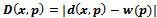where is the Euclidean distance. Similarly, Voronoi diagrams on multiplicatively weighted distances have also been studied and have numerous applications[3].

We know turn our attention to a set of the Laguerre distance functions [5]. From this definition it is clear that the Euclidean metric corresponds to the Laguerre metric when. The focus of this section will be on the metric (more commonly known as the Taxicab or Manhattan metric) and the additively weighted metric known as the power distance, which generalizes the Voronoi diagram to higher dimensions[5]. The main features and properties of the Voronoi diagram will be discussed; however, their computations are omitted.

4.1. Taxicab Metric

The taxicab metric is motivated by the layout of streets in an urban area, which tend to form an orthogonal grid. In this model the distance between two sites is taken to be the absolute difference of their coordinates. That is, if and are points in the Euclidean plane, then their taxicab distance is defined by [6].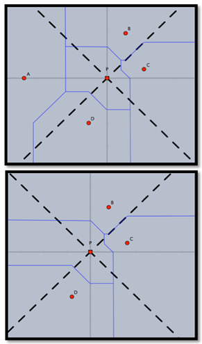

Figure 6. Boundedness of Voronoi cells in the Taxicab metric. Red points are sites, blue lines are Voronoi edges, the shaded grey lines are the coordinate axes, and the black dotted lines through P have slope of magnitude. Notice each point lie in different half planes bounded by the black dotted lines, and in the first picture, the Voronoi cell of P is bounded. The second picture illustrates how the removal of any of , or, results in an unbounded Voronoi cell (with respect to the half plane that the removed point was formally in)

One way to visualize the Voronoi diagram of point sites in the Euclidean metric is to grow circles of equal radii centered at each point site. The intersection of the circles will then trace out the edges of the Voronoi diagram. This stems from the fact that locus of points of equal distance to a single point p lie on a circle centred at p. This same concept can be applied in the Taxicab metric wherein a circle is defined as a square that is rotated to the coordinate axis[6].

The mid-set of two point sites in the Taxicab Metric takes one of three forms[6]. Let be the line segment between two site points in the Euclidean plane. If is parallel to the coordinate axis, then the mid-set corresponds to the Euclidean perpendicular bisector and is either a vertical or horizontal line. If the absolute value of the slope of is less than 1, then the mid-set has three parts: two vertical opposite rays connected by a line segment that is to the coordinate axes. Symmetrically, if the absolute value of the slope is greater than 1 then the mid-set is composed of two horizontal vertical rays connected by a line segment that is to the coordinate axes. Finally, if the slope of is exactly 1 then the mid-set contains two disjoint areas connected by a line segment that is to the coordinate axis. Hence most algorithms that compute the Voronoi diagram using the Taxicab distance require that the segment between any two sites cannot have a slope of 1. This can be done by perturbing two sites in the same way it was done for line segments sharing an endpoint.

It is clear that the Voronoi diagram in the Taxicab metric will consist of lines and line segments that are either parallel or at a angle to the coordinate axis. Voronoi Vertices are the centres of Taxicab circles passing through exactly three sites (assuming that no four sites lie on the same empty Taxicab circle).

While the point sites on the convex hull have unbounded cells in the Taxicab metric, point sites inside the convex hull aren’t necessarily bounded. Consider a site p and the lines through p with slope -1 and 1. These lines subdivide the plane into 4 open regions. By the definition given above of mid-sets, it is clear that the Voronoi cell of p is unbounded if and only if at least one of the open regions described above contains no other site q. Otherwise is bounded. Figure 6 illustrates this property.

4.2. Power Diagrams and Laguerre Geometry

The Power diagram is a very important generalization of the Voronoi diagram of circular sites. In this model we consider point sites with additive weights (also known as a site’s generating circle). The distance function used is 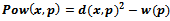. Hence each site can be interpreted as a sphere:

[5].

Voronoi edges and Vertices are defined in terms of two circle’s radical axis and their radical centres respectively. The radical axis is the points of equal power-distance from two circles, and the radical centre is the intersection of three radical axes. It follows that the Voronoi cell of a site p is [5]. If every site has equal weight, then the Power diagram corresponds to the Voronoi diagram of the point set.

What is particularly nice about the Power diagram is the fact that sets of points of equal distance between sites are linear. The radical axis of two sites p and q is perpendicular to the segment but is different from the perpendicular bisector due to the additive weights. If two generating circles intersect at one or two points then the radical axis will pass through their intersection points.

There are a variety of notable attributes of Voronoi cells in the Power diagram. While the convexity of Voronoi cells is maintained in the Power diagram, some cells may be empty (as a result of a site’s generating circle being contained within the union of other site’s generating circles). Sites that have non-empty Voronoi cells generate substantial circles, while those that do not, generate trivial circles. While sites that generate substantial circles are internal to their Voronoi cell, parts of their generating circle may be external (e.g. in the case that two generating circles intersect). Finally, a non-empty Voronoi cell is bounded if and only if p is on the boundary of the convex hull of P. While the computation of the Power diagram will not be discussed here, it should be noted that it’s time complexity in two dimensions is , and there exists algorithms for higher dimensions that can be computed in [5].

5. Conclusions

The 1^st-order Voronoi diagram of a point set generalizes naturally to a variety of different structures. The generalizations outlined in this paper are by no means an exhaustive list, but nevertheless serve to develop a flavour of the questions one must consider when generalizing the Voronoi diagram’s elementary properties to different structures. The questions that arise in almost all cases have to deal with the definition of mid-set between two objects. It has been shown that the mid-set can easily become quite complex and imposes restrictions on the set of sites we are interested in. Likewise, the computation and storage of Voronoi diagrams can become quite cumbersome which give rise to simplification of some models and approximations of the Voronoi diagram.

ACKNOWLEDGEMENTS

Dr. Vassilev’s research is supported by NSERC Discovery Grant. Brian Eades would like to acknowledge the support and guidance of Dr.Vassilev throughout the work on this research. We also would like to thank the two anonymous referees for their useful suggestions aimed at improving the paper.