-
Paper Information
- Paper Submission
-
Journal Information
- About This Journal
- Editorial Board
- Current Issue
- Archive
- Author Guidelines
- Contact Us
American Journal of Computational and Applied Mathematics
p-ISSN: 2165-8935 e-ISSN: 2165-8943
2013; 3(2): 49-67
doi:10.5923/j.ajcam.20130302.01
A Random-effects Regression Specification Using a Local Intercept Term and a Global Mean for Forecasting Malarial Prevalance
 Abstract
 Reference
 Full-Text PDF
 Full-text HTML
Benjamin G. Jacob1, Ranjit de Alwiss2, Semiha Caliskan1, Daniel A. Griffith3, Dissanayake Gunawardena4, Robert J. Novak1
1Global Infectious Disease Research Program, Department of Public Health, College of Public Health, University of South Florida, 3720 Spectrum Blvd, Suite 304, Tampa, Florida, USA 33612
2Abt Associates Inc. Uganda IRS Project, Plot 33, Yusuf Lule Road, Kampala P. O.Box 37443, Uganda
3School of Economic, Political and Policy Sciences. The University of Texas as Dallas, 800 West Campbell Road, Richardson, TX 75080-3021
4USAID Presidents Malaria incentive (PMI), Uganda
Correspondence to: Benjamin G. Jacob, Global Infectious Disease Research Program, Department of Public Health, College of Public Health, University of South Florida, 3720 Spectrum Blvd, Suite 304, Tampa, Florida, USA 33612.
| Email: |  |
Copyright © 2012 Scientific & Academic Publishing. All Rights Reserved.
Historically, malaria disease mapping has involved the analysis of disease incidence using a prevalence responsible variable often available as aggregate counts over a geographical region subdivided by administrative boundaries (e.g., districts). Thereafter, commonly, univariate statistics and regression models have been generated from the data to determine covariates (e.g., rainfall) related to monthly prevalence rates. Specific district-level prevalence measures however, can be forecasted using autoregressive specifications and spatiotemporal data collections for targeting districts that have higher prevalence rates. In this research, initially, case, as counts, were used as a response variable in a Poisson probability model framework for quantifying datasets of district-level covariates (i.e., meteorological data, densities and distribution of health centers, etc.) sampled from 2006 to 2010 in Uganda. Results from both a Poisson and a negative binomial (i.e., a Poisson random variable with a gamma distrusted mean) revealed that the covariates rendered from the model were significant, but furnished virtually no predictive power. Inclusion of indicator variables denoting the time sequence and the district location spatial structure was then articulated with Thiessen polygons which also failed to reveal meaningful covariates. Thereafter, an Autoregressive Integrated Moving Average (ARIMA) model was constructed which revealed a conspicuous but not very prominent first-order temporal autoregressive structure in the individual district-level time-series dependent data. A random effects term was then specified using monthly time-series dependent data. This specification included a district-specific intercept term that was a random deviation from the overall intercept term which was based on a draw from a normal frequency distribution. The random effects specification revealed a non-constant mean across the districts. This random intercept represented the combined effect of all omitted covariates that caused districts to be more prone to the malaria prevalence than other districts. Additionally, inclusion of a random intercept assumed random heterogeneity in the districts’ propensity or, underlying risk of malaria prevalence which persisted throughout the entire duration of the time sequence under study. This random effects term displayed no spatial autocorrelation, and failed to closely conform to a bell-shaped curve. The model’s variance, however, implied a substantial variability in the prevalence of malaria across districts. The estimated model contained considerable overdispersion (i.e., excess Poisson variability): quasi-likelihood scale = 76.565. The following equation was then employed to forecast the expected value of the prevalence of malaria at the district-level: prevalence = exp[-3.1876 + (random effect)i] . Compilation of additional and accurate data can allow continual updating of the random effects term estimates allowing research intervention teams to bolster the quality of the forecasts for future district-level malarial risk modelling efforts.
Keywords: Poisson Variability, Prevalence, Random Effects, Malaria Autoregressive Integrated Moving Average, Autocorrelation
Cite this paper: Benjamin G. Jacob, Ranjit de Alwiss, Semiha Caliskan, Daniel A. Griffith, Dissanayake Gunawardena, Robert J. Novak, A Random-effects Regression Specification Using a Local Intercept Term and a Global Mean for Forecasting Malarial Prevalance, American Journal of Computational and Applied Mathematics , Vol. 3 No. 2, 2013, pp. 49-67. doi: 10.5923/j.ajcam.20130302.01.
Article Outline
1. Introduction
- Ecological regression for malaria disease mapping mainly focuses on simulating estimation of risk in administrative regions which are commonly exploited using Poisson specifications[1]. A discrete stochastic variable X is said to have a Poisson distribution with parameter λ>0, if k = 0, 1, 2, while the probability mass function of X is rendered by:
 where e is the base of the natural logarithm (e = 2.71828...) and k! is the factorial of k[2]. The mode of a Poisson-distributed malaria-related sampled variable with a non-integer λ is then equal to
  which in turn will represent the largest integer less than or equal to λ in the model. This can also be written as floor (λ).The floor function
  then would be the greatest integer function or integer value generating the largest integer less than or equal to x. Commonly, the floor and ceiling functions then maps a field-sampled malarial- related covariate coefficient value to the largest previous or the smallest following integer, respectively, where floor(x) =
  and is the largest integer not greater than x and ceiling(x) =
  is the smallest integer not less than x[1]. Since λ would be a positive integer in a spatiotemporal sampled district-level malaria regression-based model, for example, the modes would be λ and λ – 1. By so doing, all of the cumulants of the Poisson distribution in the malarial model would be equal to the expected value λ calculated at each sampled district-level location.Further, the explanatory predictor covariate coefficient of variation in a Poisson-specified malaria-related regression model would then be
  while the index of dispersion would be 1. Thereafter, commonly, the mean deviation about the mean in the district-level malarial model would be expressed as
  for determining statistical significance of the spatiotemporal sampled parameter estimators. On occasion the negative binomial distribution can be used as a substitute to the Poisson distribution especially in its alternative parameterization state. This distribution may be especially useful for time series-dependent malarial- related discrete data over an unbounded positive range whose sample variance exceeds the sample mean. In such cases, the observations would be overdispersed with respect to a Poisson distribution, for which traditionally, the mean is equal to the variance. Additionally, spatial statistics has recently provided new methodologies and solutions for invasive residual autoregressive uncertainty diagnostic analyses (e.g., derivation of eigenvalues of second order coupled with differential equations) employingspatiotemporal sampled malarial-related explanatory covariate coefficient estimates[1]. Recent advances in local spatial statistics have led to a growing interest in the detection of disease clusters or 'hot spots', for public health surveillance for improving disease etiology and the pathogenesis of epidemics such as malaria. For example, Moran’s I is a global parameter for the measurement of autocorrelation, which can be used to examine individual seasonal-sampled district-level geographical locations enabling “hotspots” to be identified based on comparison with neighbouring sampled district- level malarial-related data feature attributes. Moran's I is a measure of spatial autocorrelation which in seasonal malaria modelling is characterized by a correlation in a signal among nearby sampled data locations in space[1]. Hot spot cluster analyses can be an effective methodology for defining elevated concentrations of an environmental phenomenon[2]. Among a few methods proposed for hotspot or spatial cluster identification is the Moran's I which is a measure of spatial autocorrelation. Spatial autocorrelation is the correlation among values of a single variable strictly attributable to their relatively close geographical locational positions on a two-dimensional surface, introducing a deviation from the independent observations assumption of classical statistics[3]. Often spatial autocorrelation used in mathematical spatiotemporal arthropod-born infectious disease analyses is characterized by a correlation in a signal among nearby larval habitat locations in geographical space such as Getis’G index, spatial scan statistics, and Tango’s C index but, currently the local Moran’s I index is the most popular index[1].In this research our assumption was that by calculating analytic derivatives with line parameter restrictions and estimation of simultaneous systems using linear and non-linear regression-based algorithmic equations with distributed lags and time-series dependent error quantification processes, robust spatial forecasts of district-level malaria-related prevalence rates could be generated. Thereafter, by analysing and identifying the spatiotemporal sampled covariate coefficient estimates as delineated by our model residuals, we assumed we could elucidate mechanisms for accurately predicting underlying district-level geographic locations of higher prevalence rates (e.g., higher monthly precipitation values, higher urban populations). Mathematical malarial regression models should focus on treatment based on surveillance of the most productive areas of an ecosystem[4].Another assumption in this research was that we could use the mathematically predicted prevalence rates from the linear and spatial autoregressive risk distribution model outputs for implementing cost-effective larval control measures throughout Uganda. For example, in theory, georeferenced explanatory covariate coefficients rendered from a stochastic robust interpolator could predicatively map, district-level regions that have higher prevalence rates for targeting areas and/or feature data attributes that contribute to areas of greater rates. Since the devastating situation of malaria in Uganda can be explained to a large e xtent by the mounting drug-resistance problem and the lack of a vaccine[4], an integrated mathematical-based predictive map targeting geographic locations may reveal sound understanding of district-level malarial transmission dynamics especially in highly populated urban regions. The importance of this work may also be expressed in mathematical literature regarding representations of geographic space. Therefore, the objectives of this research were to: (1) construct a robust Poisson regression model framework using multiple field and remote-sampled predictor variables; (2) generate a spatial autoregressive- oriented error matrix using the estimators; 3) filter all latent autocorrelation parameters in the residual variance employing an eigenfunction decomposition algorithm to accurately forecast district-level malarial rates by eliminating the effect of variables' uncertainties(e.g., perfect multicollinearity) in multiple spatiotemporal empirical ecological datasets of district-level time-series dependent georeferenced explanatory covariate coefficients seasonally - sampled from 2006 to 2010 in Uganda.
2. Materials and Methodology
2.1. Study Site
- Uganda is a landlocked country in East Africa. The country is located on the East African plateau, lying mostly between latitudes 4°N and 2°S (a small area is north of 4°), and longitudes 29° and 35°E. It averages about 1,100 meters (3,609 ft.) above sea level, and this slopes very steadily downwards to the Sudanese Plain to the north. However, much of the south is poorly drained, while the center is dominated by Lake Kyoga, which is also surrounded by extensive marshy areas. In many hyperendemic areas, malaria prevalence in communities is maximum in areas bordering on marshes where rates can range from 1% to 15% according to age and season of the year[4].Although generally equatorial, the climate is not uniform as the altitude modifies the climate. Southern Uganda is wetter with rain generally spread throughout the year. At Entebbe on the northern shore of Lake Victoria, most rain falls from March to June and in the November/December period. Further to the north a dry season gradually emerges, for example, at Gulu about 120 km from the South Sudanese border where November to February is much drier than the rest of the year. Uganda is divided into districts spread across four administrative regions: Northern, Eastern, Central (i.e., Kingdom of Buganda) and Western. The districts are subdivided into counties. A number of districts have been added in the past few years, and eight others were added on July1, 2006 plus others were added throughout 2010. There are presently over 100 districts. Most districts are named after their main commercial and administrative towns. Each district is divided into sub-districts, counties, sub-counties, parishes and villages. See Figure 1 for district-level administrative divisions in Uganda.
2.2. Environmental Parameters
- Initially, the data analysis explored covariation between prevalence[i.e., (adjusted cases)/population, which in this research was not the same as the reported number of probable and confirmed cases], variable Y, and the following variables: annual—population density, density of clinics, and density of water bodies; monthly—humidity, rainfall and vegetation indices.
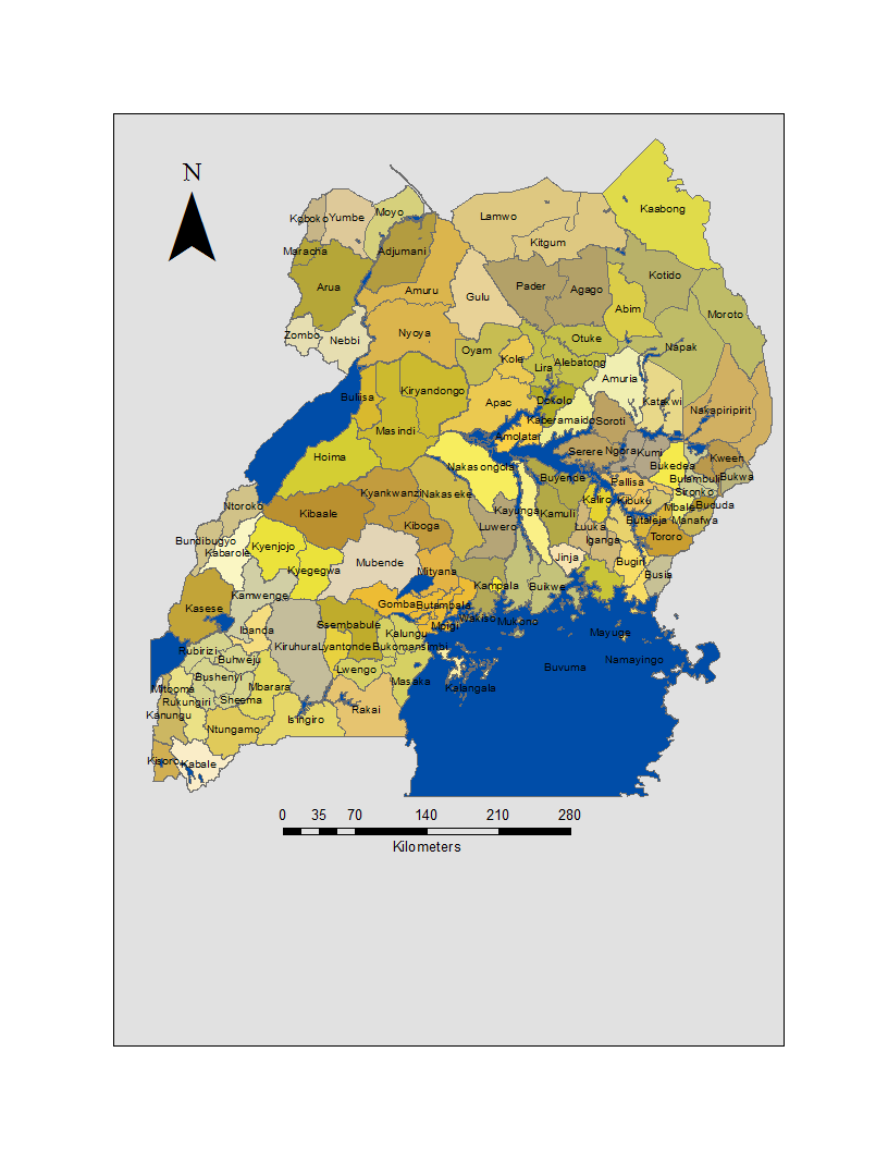 | Figure 1. Administrative Boundaries: of districts in Uganda |
2.3. Regression Model
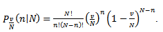
- We then constructed a Poisson model in SAS GEN MOD. The Poisson process in our analyses was provided by the limit of a binomial distribution of the sampled district-level explanatory predictor covariate coefficient estimates using
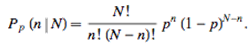 | (2.1) |
 Based on the sample size N, the distribution approached
  was
was 
 The GENMOD procedure then fit a generalized linear model (GLM) to the sampled data by maximum likelihood estimation of the parameter vector β. In this research the GENMOD procedure estimated the seasonal-sampled parameters of each district-level malaria model numerically through an iterative fitting process. The dispersion parameter was then estimated by the residual deviance and by Pearson’s chi-square divided by the degrees of freedom (d.f.). Covariances, standard errors, and p-values were then computed for the sampled covariate coefficients based on the asymptotic normality derived from the maximum likelihood estimation.Note, that the sample size N completely dropped out of the probability function, which in this research had the same functional form for all the sampled district-level parameter estimator indicator values (i.e.,
  ). As expected, the Poisson distribution was normalized so that the sum of probabilities equaled 1. The ratio of probabilities was then determined by
 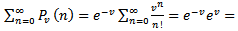 which was then subsequently expressed as
 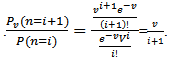 The Poisson distribution revealed that the explanatory covariate coefficients reached a maximum when
 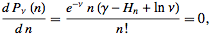 where
where  was the Euler-Mascheroni constant and
  was a harmonic number, leading to the transcendental equation
 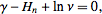 . The regression model also revealed that the Euler-Mascheroni constant arose in the integrals as
 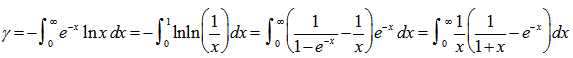 | (2.2) |
 in combination with temporal sampled constants include
 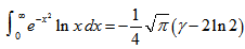 which is equal to
 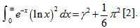 Thereafter, the double integrals in our district-level seasonal malaria regression model included
 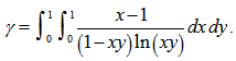 An interesting analog of equation (2.2) in the regression-based model was then calculated as
  . This solution was also provided by incorporating Mertens theorem[i.e.,
 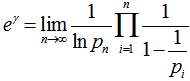 where the product was aggregated over the district-level sampled values found in the empirical ecological datasets. IMertens' 3rd theorem:
 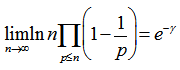 is related to the density of prime numbers where γ is the Euler–Mascheroni constant[5].By taking the logarithm of both sides in the model, an explicit formula for γ was then derived employing
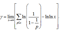 . This expression was also rendered coincidently by quantifying the data series employing Euler, and equation (2.2) by first replacing
  , in the equation
 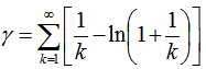 and then generating
  . We then substituted the telescoping sum
  which then generated
  . Thereafter, our product was
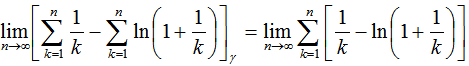 .Additionally, other series in our spatiotemporal district-level regression model included the equation (◇) where
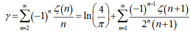 and
and  was
was 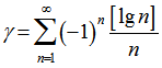 plus the Riemann zeta function. The Riemann zeta function ζ(s) is a function of a complex variables that analytically continues the sum of the infinite series
  which converges when the real part of s is greater than 1 where lg is the logarithm to base 2 and the
  is the floor function[2]. Nielsen[5] earlier provided a series equivalent to
 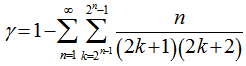 and, thereafter
  which was then added to
  to render Vacca's formula. Gosper et al.[6] used the sums
 with
with  by replacing the undefined I and then rewrote the equation as a double series for applying the Euler's series transformation to each of the sampled time-series dependent explanatory covariate coefficient estimates.In this research
  was used as a binomial coefficient, rearranged to achieve the conditionally convergent series in our spatiotemporal district-level linear model. The plus and minus terms were first grouped in pairs of the sampled covariate coefficient estimates employing the resulting series based on the actual observational covariate coefficient indicator values. The double series was thereby equivalent to Catalan's integral:
  . Catalan's integrals are a special case of general formulas due to
 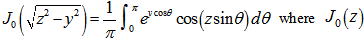 is a Bessel function of the first kind[3]. The Bessel function is a function
  defined in a robust regression model by using the recurrence relations
 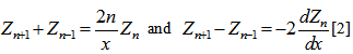 which more recently has been defined as solutions in linear models using the differential equation
 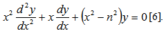 In this research the Bessel function
  was defined by the contour integral
 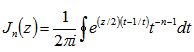 where the contour enclosed the origin and was traversed in a counter-clockwise direction. This function generated:
  In mathematics, Bessel functions are canonical solutions y(x) of Bessel's differential equation:
 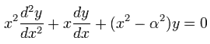 for an arbitrary real or complex number α (i.e., the order of the Bessel function); the most common and important cases are for α an integer or half-integer[2]. Thereafter, to quantify the equivalence in the spatiotemporal malarial regression-based parameter estimators, we expanded
  in a geometric series and multiplied the district-level sampled data feature attributes by
 , and integrated the term wise as in Sondow and Zudilin[6].Other series for
 then included
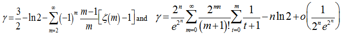 A rapidly converging limit for
  was then provided by
 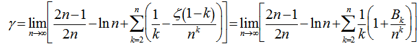 and
and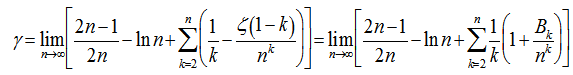 where
where  was a Bernoulli number. Another limit formula was then provided by the equation
  In mathematics, the Bernoulli numbers Bn are a sequence of rational numbers with deep connections to number theory, whereby, values of the first few Bernoulli numbers are B0 = 1, B1 = ±1⁄2, B2 = 1⁄6, B3 = 0, B4 = −1⁄30, B5 = 0, B6 = 1⁄42, B7 = 0, B8 = −1⁄30[2]. Jacob et al.[1] found if m and n are sampled values and f(x) is a smooth sufficiently differentiable function in a seasonal malarial-related regression model which is defined for all the values of x in the interval
  then the integral
  can be approximated by the sum (or vice versa)
  . The Euler–Maclaurin formula then provided expressions for the difference between the sum and the integral in terms of the higher derivatives ƒ(k) at the end points of the interval m and n. The Euler–Maclaurin formula provides a powerful connection between integrals and sums which can be used to approximate integrals by finite sums, or conversely to evaluate finite sums and infinite series using integrals and the machinery of calculus[5]. Thereafter, for the district-level malarial-sampled values, p, we had
  where B1 = −1/2, B2 = 1/6, B3 = 0, B4 = −1/30, B5 = 0, B6 = 1/42, B7 = 0, B8 = −1/30, and R which was an error term. Note in this research
  Hence, we re-wrote the regression-based formula as follows:
  We then rewrote the equation more elegantly as
  with the convention of
  (i.e. the -1th derivation of f is the integral of the function). Limits to the district-level malaria regression model was then rendered by
  where
where  was the Riemann zeta function. The Bernoulli numbers appear in the Taylor series expansions of the tangent and hyperbolic tangent functions, in formulas for the sum of powers of the first positive integers, in the Euler–Maclaurin formula and in expressions for certain values of the Riemann zeta function[2].Another connection with the primes was provided by
  for the sampled district-level numerical values from 1 to
  in the spatiotemporal sampled malarial dataset which in this research was found to be asymptotic to
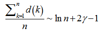 . De laValléePoussin[7] proved that if a large number n is divided by all
  , then the average amount by which the quotient is less than the next whole number is g[2]. An identity for g in our malaria district-level regression-based model was then provided by
 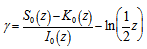 where
where  was a modified Bessel function of the first kind,
  was a modified Bessel function of the second kind, and
 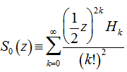 where
where  was a harmonic number. For non-integer α, Yα(x) is related to Jα(x) by:
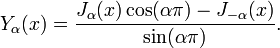 In the case of integer order n, the function is defined by taking the limit as a non-integer α tends to n:
  [2]. In this research, the Bessel functions of the second kind, were denoted by Yα(x), and by Nα(x), which were actually solutions of the Bessel differential equation employing a singularity at the origin (x = 0).This provided an efficient iterative algorithm for g by computing
 and
and Reformulating this identity rendered the limit
  Infinite products involving g also arose from the Barnes G-function using the positive integer n. In mathematics, the Barnes G-function G(z) is a function that is an extension of superfactorials to the complex numbers which is related to the Gamma function[3]. In this research, this function provided
  and also the equation
 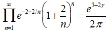 . The Barnes G-function was then linearly defined in our time-series dependent district-level malarial regression-based model which then generated
 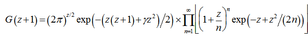 where γ was the Euler–Mascheroni constant, exp(x) = ex, and ∏ was capital pi notation. The Euler-Mascheroni constant was then rendered by the expressions
  where
where  was the digamma function
  and the asymmetric limit form of
 In mathematics, the digamma function is defined as the logarithmic derivative of the gamma function:
  where it is the first of the polygamma functions. In our model the digamma function, ψ0(x) was then related to the harmonic numbers in that
  where Hn was the nth harmonic number, and γ was the Euler-Mascheroni constant. In mathematics, the n-th harmonic number is the sum of the reciprocals of the first n natural numbers[2].The difference between the nth convergent in equation (◇) and
  in our district-level regression-based model was then calculated by
  where
where  was the floor function which satisfied the inequality
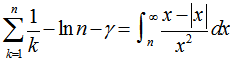 . The symbol g was then
 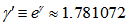 . This led to the radical representation of the sampled district-level covariate coefficients as
 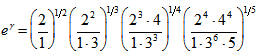 which was related to the double series
 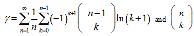 a binomial coefficient.Thereafter, another proof of product in the our spatiotemporal district-level malarial regression model was provided by the equation
 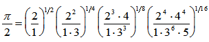 . The solution was then made even clearer by changing
  . In this research, both these regression-based formulas were also analogous to the product for
  which was then rendered by calculating
 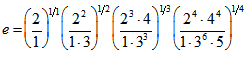 .
.2.4. Negative Binomial Regression
- Unfortunately, extra-Poisson variation was detected in the variance estimates in our model. A modification of the iterated re-weighted least square scheme and/or a negative binomial non-homogenous regression-based framework conveniently accommodates extra-Poisson variation when constructing seasonal log-linear models employing frequencies or prevalence rates as dependent response variables[2].Operationally these models consists of making iterated weighted least square fit to approximately normally distributed dependent malarial-related explanatory predictor covariate coefficients based on observed rates or their logarithm. Unfortunately, the variance of malarial-related observations in log-linear equations are commonly assumed to be constant[1].Subsequently, introducing an extra-binomial variation scheme in a malarial-related linear-logistic model can be fitted for a Poisson procedure. The probabilities describing the possible outcome of a single trial are modeled, as a function of explanatory predictor variables, using a logistic function[2].As such, we constructed a robust negative binomial regression model in SAS with non-homogenous means and a gamma distribution by incorporating
 in equation (2.1) . We let
  be the probability density function of
  in the model. Then, the distribution
  was no longer conditional on
  . Instead it was obtained by integrating
  with respect to
  :
:  . The distribution in the linear district-level malaria regression model was then
 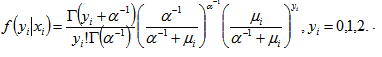 The negative binomial distribution was thus derived as a gamma mixture of Poisson random variables. The conditional mean in the model was then
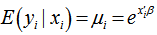 and the variance in the residual estimates was.
 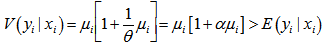 To further estimate the district-level models, we specified DIST=NEGBIN (p=1) in the MODEL statement in PROC REG. The negative binomial model NEGBIN1 was set p=1 , which revealed the variance function
 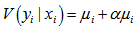 was linear in the mean of the model. The log-likelihood function of the NEGBIN1 model was then provided by
 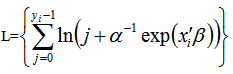 Additionally, the equation
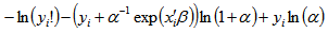 was generated. The gradient for our spatiotemporal malarial-based regression model was then quantified employing
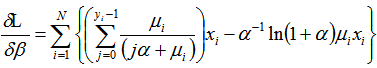 and
and 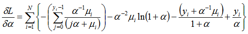 In this research, the negative binomial regression model with variance function
 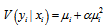 , was then referred to as the NEGBIN2 model. To estimate this regression-based model, we specified DIST=NEGBIN (p=2) in the MODEL statements. A test of the Poisson distribution was then performed by examining the hypothesis that
  . A Wald test of this hypothesis was also provided which were the reported t statistics for the estimates in the model. Under the Wald statistical test, the maximum likelihood estimate
  of the parameter(s) of interest
  is compared with the proposed value
  , with the assumption that the difference between the two will be approximately normally distributed[2]. The log-likelihood function of the regression models (i.e., NEGBIN2) was then generated by the equation:
 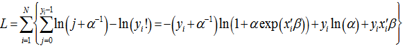 whose gradient was
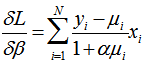 . The variance in our model was then assessed by
 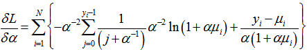 . The final mean in the model was calculated as:
  , the mode as;
 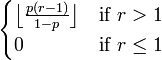 , the variance as
  , the skewess as
  , the kurtosis as
  , the moment generating function as
 , the characteristic function as
  ; and, the probability generating function as
  .
. 2.5. Autocorrelation Model
- A spatial autoregressive model was then generated that used a variable Y, as a function of nearby sampled district–level covariate coefficients. In this research, Y had an indicator value 1 (i.e., an autoregressive response) and/or the residuals of Y which were values of nearby sampled Y residuals (i.e., an SAR or spatial error specification). For time series-dependent modelling malaria-related parameter estimators, the SAR model furnishes an alternative specification that frequently is written in terms of matrix W[1]. A misspecification perspective was then used for performing a spatial autocorrelation uncertainty estimation analyses using the sampled district-level covariates. The model was built using the
 (i.e. regression equation) assuming the sampled data had autocorrelated disturbances. The model also assumed that the sampled data could be decomposed into a white-noise component,
  , and a set of unspecified sub-district level malarial regression models that had the structure
 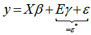 . Jacob et al.[1] found that white noise in a seasonal malaria-based regression model is a univariate or multivariate discrete-time stochastic process whose terms are independent and independent (i.i.d) with a zero mean. In this research, the misspecification term was
3. Results
- Initially, we constructed a Poisson regression model using the spatiotemporal seasonal-sampled district-level covariate coefficient measurement values. Our model was generalized by introducing an unobserved heterogeneity term for each sampled district-level observation
 . The weights were then assumed to differ randomly in a manner that was not fully accounted for by the other seasonal-sampled covariates. In this research this district-level process was formulated as
 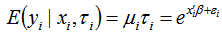 where the unobserved heterogeneity term
  was independent of the vector of regressors
  . Then the distribution of
  was conditional on
  and had a Poisson specification with conditional mean and conditional variance
 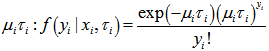 . We then let
  be the probability density function of
  . Then, the distribution
  was no longer conditional on
  Instead it was obtained by integrating
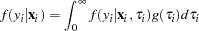
  with respect to
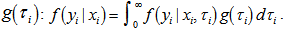 We found that an analytical solution to this integral existed in our district-level malaria model when
  was assumed to follow a gamma distribution. The model also revealed that
  , was the vector of the sampled predictor covariate coefficients while
  , was independently Poisson distributed with
 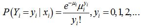 and the mean parameter — that is, the mean number of district-level sampling events per spatiotemporal period — was given by
  where
where was a
was a  parameter vector. The intercept in the model was then
  and the coefficients for the
  regressors were
  Taking the exponential of
  ensured that the mean parameter
  was nonnegative. Thereafter, the conditional mean was provided by
 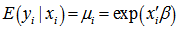 .The district-level parameter estimators were then evaluated using
 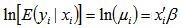 . Note, that the conditional variance of the count random variable was equal to the conditional mean (i.e., equidispersion) in our model[i.e., ,
 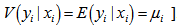 . In a log-linear model the logarithm of the conditional mean is linear[2]. The marginal effect of any district-level regressor in the malarial model was then provided by
 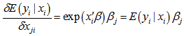 . Thus, a one-unit change in the
  th regressor in the model led to a proportional change in the conditional mean
  . In this research, the standard estimator for our Poisson model was the maximum likelihood estimator. Since the district-level observations were independent, the log-likelihood function in the model was then:
 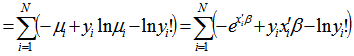 . Given the sampled dataset of district-level parameter estimators (i.e., θ ) and an input vector x, the mean of the predicted Poisson distribution was then provided by
 . By so doing, the Poisson distribution's probability mass function was then rendered by
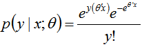 The probability mass function in a targeted spatiotemporal predictive seasonal malaria risk model can be the primary means for defining a discrete probability distribution, and, as such, functions could exist for either scalar or multivariate field-sampled random variables, given that the distribution is discrete.[1] Gu and Novak[4] found that a targeted spatiotemporal predictive seasonal malaria risk model is vital for district level larval control interventions.Since in this research, the sampled data consisted of m vectors
 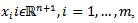 , along with a set of m values
  then, for the sampled parameter estimators θ, the probability of attaining this particular set of the sampled observations was provided by the equation
 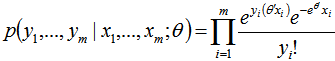 .Consequently, we found the set of θ that made this probability as large as possible in the model estimates. To do this, the equation was first rewritten as a likelihood function in terms of θ:
 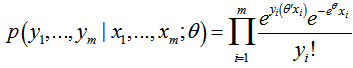 .Note the expression on the right hand side in our model had not actually changed. Next, we used a log-likelihood[i.e.,
 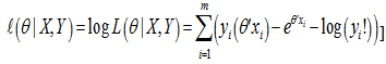 . Because the logarithm is a monotonically increasing function, the logarithm of a function achieves its maximum value at the same points as the function itself, and, hence, the log-likelihood can be used in place of the likelihood in maximum likelihood estimation and related techniques[2]. Finding the maximum of a function in a malarial-related model often involves taking the derivative of a function and solving for the parameter estimator being maximized, and this is often easier when the function being maximized is a log-likelihood rather than the original likelihood function [1].Notice that the parameters θ only appeared in the first two terms of each term in the summation. Therefore, given that we were only interested in finding the best value for θ in the district-level predictive malarial-related regression model we dropped the yi! and simply wrote
 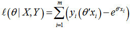 . Thereafter, to find a maximum, we solved an equation
  which had no closed-form solution. However, the negative log-likelihood (LL)[i.e.,
  ] was a convex function, and so standard convex optimization was applied to find the optimal value of θ .We found that given the Poisson process in our regression model the limit of a binomial distribution was
 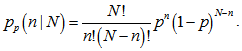 Viewing the distribution as a function of the expected number of successes[i.e.,
  ] in the model, instead of the sample size N for fixed P, then rendered the equation (2.1) which then became
 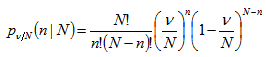 Our model revealed that as the sample size N become larger, the distribution approached P when the following equations aligned
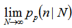

 . Note, in this research, that the sample size N had completely dropped out of the probability function, which had the same functional form for all values of
  in the model. Thereafter, as expected, the Poisson regression distribution was normalized so that the sum of probabilities was equal to 1, since
  The ratio of probabilities was then provided by the equation
  . Our model revealed that the Poisson distribution reached a maximum when
 where g was the Euler-Mascheroni constant and
  was a harmonic number, leading to the equation
  which could not be solved exactly for n.Next, the moment-generating function of the Poisson distribution was given by
 , when
  ,
, so
so  . The raw moments were also computed directly by summation, which yielded an unexpected connection with the exponential polynomial
  and Stirling numbers of the second kind[i.e.
  which in this research was the Dobiński's formula.In combinatorial mathematics, Dobinski’s formula states that the number of partitions of a set of n members is
  This number has come to be called the nth Bell numberBn, where the proof is rendered as an adaptation to probabilistic language as given by Rota[11]. In our malarial-based regression model the formula
  was then viewed as a particular case, for x=0, employing the relation
  . The expression given by the model’s Dobinski's formula was then revealed as the n th moment of the Poisson distribution with expected value 1. In this research, Dobinski's formula was the number of partitions of a set of the sampled malarial parameter estimator size (i.e.,n) which equalled the nth moment of that distribution. We used the Pochhammer symbol (x)n to denote the falling factorial
 . If x and n are nonnegative integers, 0 ≤ n ≤ x, then (x)n is the number of one-to-one functions that map a size-n set into a size-x set[1]. At this junction we let ƒ be any function from a size-n set A into a size-x set B. Thus, in the model. u ∈ B .We then let ƒ−1(u) = {v ∈ A : ƒ(v) = u}. Then {ƒ−1(u) : u ∈ B} was a partition of A. This equivalence relation was the "kernel" of the function ƒ. Any function from A into B factors in to one function that maps a member of A to that part of the kernel to which it belongs, and another function, which is necessarily one-to-one, that maps the kernel into B[2]. In this research the first of these two factors was completely determined by the partition π, that is the kernel. The number of one-to-one functions from π into B was then (x)|π|, in the district-level malarial regression model when |π| was the number of parts in the partition π. Therefore, the total number of functions from a size-n set A into a size-x set B was
  in the model when the index π ran through the set of all partitions of A. On the other hand, the number of functions from A into B was clearly xn. Thus, we had
  Since X was a Poisson-distributed spatiotemporal-seasonal malarial-related district-level random variable with expected value 1, then the nth moment of this probability distribution was
 but all of the factorial moments E((X)k) of this probability distribution was equal to 1 in the model also. Thereafter, we had,
  ,which was the number of partitions of the set A in the model. Therefore, in the model,
  , and
, and  .Thereafter, the central moments in the malarial model was computed as
  so the mean, variance, skewness, and kurtosis were
 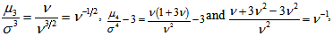 respectively. The characteristic function for the Poisson distribution in the district -level Poisson predictive autoregressive model was then revealed as
  and the cumulative distribution function was
  so
so  The mean deviation of the Poisson distribution mode was then rendered by
 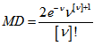 . The cumulative distribution functions of the Poisson and chi-squared distributions were then related in the district-level model as
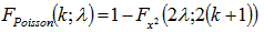 integer k and
 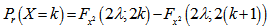 . The Poisson distribution was then expressed in terms of
  whereby, the rate of changes were equal to the equation
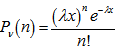 . The moment-generating function of the Poisson distribution generated from the sampled district-level explanatory predictor variables was also rendered by
  Given a random variable x and a probability distribution function
  , if there exists an
  such that
  , where
  denotes the expectation value of
  , then
  is called the moment-generating function[2]. Commonly, for a continuous distribution in a seasonal linear regression-based time-series dependent regression model
  the equation
  is used where
  the r the raw moment.[5]. For quantifying independent X and Y, the moment-generating function in a robust model must satisfy the equation
  and
and  if, the independent variables
  have Poisson distributions with parameters
  and
and  [3].In this research this was evident since the cumulant-generating function was
 .In the malaria model the directed Kullback-Leibler (K-L) divergence between Pois(λ) and Pois(λ0) was then provided by
  . In probability theory and information theory, the K-L divergence along with information divergence, information gain, relative entropy are a non-symmetric measures of the difference between two probability distributions P and Q in a model[2]. In this research, for quantifying the probability distributions P and Q of a sampled discrete random variable the K–L divergence was defined by
  . The model revealed that the average of the logarithmic difference between the probabilities P and Q was the average quantified using the probabilities P. The K-L divergence is only defined if P and Q both sum to 1 and if
  for any i such that
  [3]. In our district-level spatiotemporal malaria-based regression-based model, if the quantity 0 ln 0 appeared in the formula it was interpreted as zero. For distributions P and Q of the continuous random variable in the sampled datasets K-L divergence was defined to be the integral[i.e.,
 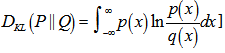 where p and q denoted the densities of P and Q. More generally, since P and Q were probability measures over the sampled dataset X, and Q which was absolutely continuous with respect to P, then the K-L divergence from P to Q was defined as
 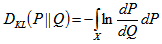 in the model where
  was the Radon–Nikodym derivative of Q with respect to P, provided the expression on the right-hand side existed. In mathematics, the Radon–Nikodym theorem is a result in measure theory that states that given a measurable space (i.e., X,Σ), if a σ-finite is measured on (i..e, X,Σ) then the expression is absolutely continuous with respect to a σ-finite measure µon (X,Σ). By so doing, in this research a measurable function f was rendered on X (0,∞), such that
 for any other measured value which then revealed the statistical significance of the sampled district-level covariate coefficients.Likewise, since P was absolutely continuous with respect to Q in the district-level malarial regression model. The explanatory predictor covariate coefficients were then defined employing:
 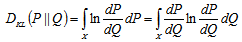 which in this research was recognized as the entropy of P relative to Q. We found that if
  was any measure on X in the model then
 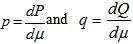 existed, and the K-L divergence from P to Q was given as
  . The bounds for the tail probabilities of the Poisson random variable were then derived in the district-level malarial regression model using a Chernoff bound argument as
 , for
, for  and as
  for
for  .In probability theory, the Chernoff bound, provides exponentially decreasing bounds on tail distributions of sums of independent random variables. It is a sharper bound than the known first or second moment based tail bounds such as Markov's inequality or Chebyshev inequality, which only yield power-law bounds on tail decay. However, in this research, the Chernoff bound required that the variates be independent - a condition that neither the Markov nor the Chebyshev inequalities require. In probability theory, Markov's inequality gives an upper bound for the probability that a non-negative function of a random variable is greater than or equal to some positive constant[5].In this research, we let X1, ..., Xn be independent Bernoulli random variables, each having probability p > 1/2. Then the probability of simultaneous occurrence of more than n/2 of the district-level sampling events had an exact value S in the model when
 The Chernoff bound revealed that S had the following lower bound:
  We noticed that if X was any sampled district-level random variable and a > 0,then
  In the language of measure theory, Markov's inequality states that if (X, Σ, μ) is a measure space, ƒ is a measurable extended real-valued function, and
  ,then
,then  [2] We then used the Chebyshev's inequality to determine the variance bound to the probability that the spatiotemporal-seasonal sampled random variable deviated far from the mean in the model. Specifically we used
  for any a>0. In this research, Var(X) was the variance of X, defined as:
  Chebyshev's inequality follows from Markov's inequality by considering the random variable
 for which Markov's inequality also reads
 [2]. Further, in Markov’s inequality if x takes only nonnegative field-sampled malarial values, then
  can be re-written
  =
= =
= However, since
  is a prevalence rate value in a spatiotemporal malarial regression-based model, it must be
  .Thus, it must be stipulated that
  so
so  =
=


 =
= =
= in order to determine district–level covariate coefficients of statistical significanceWe then considered the Euler product
 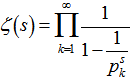 where
where  was the Riemann zeta function and
  was the k the prime.
  . Thereafter, by taking the finite product up to k=n in the district-level malarial regression model and pre-multiplying by a factor
  , we were able to employ
  to render
 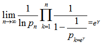 which was equivalent to 1.781072…..By doing so, g became the Euler-Mascheroni constant which in this research also represented the limit of the sequence g=
 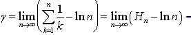 in the residuals where
  was the harmonic number which in this research had the form
  in the district-level malarial regression model. A harmonic number can be expressed analytically as
 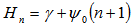 where
where  is the Euler-Mascheroni constant and
  is the digamma function[2]. Our model revealed that the Euler product attached to the Riemann zeta function
  represented the sum of the geometric series rendered from the spatiotemporal-sampled empirical dataset of explanatory predictor covariate coefficients as
 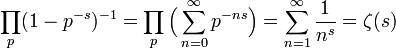 . A closely related result was also obtained by noting that
  We also considered the variation of when with the
  sign changed to a
  sign and the
  in the district-level malarial model which moved from the denominator to the numerator rendering
 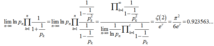 We then tested the model for overdispersion with a likelihood ratio test. This test quantified the equality of the mean and the variance imposed by the Poisson distribution against the alternative that the variance exceeded the mean. For the negative binomial distribution, the variance = mean + k mean2 (k>= 0, the negative binomial distribution reduces to Poisson when k=0)[2]. In this research, the null hypothesis was H0: k=0 and the alternative hypothesis was Ha : k>0 . To carry out the test, we used the following steps initially and then ran the model using negative binomial distribution and a record log-likelihood (LL) value. We then recorded LL for the Poisson model. We used the likelihood ratio (LR) test, that is, we computed LR statistic, -2(LL (Poisson) – LL (negative binomial). The asymptotic distribution of the LR statistic had probability mass of one half at zero and one half – chi-sq distribution with 1 d.f. To test the null hypothesis further at the significance level , we then used the critical value of chi-sq distribution corresponding to significance level 2, that is we rejected H0 if LR statistic >2 (1-2 , 1 df).Next, we assumed that our spatiotemporal sampled district-level malaria model explanatory predictor covariate coefficient estimates were based on the log of the mean, , which in this research was a linear function of independent variables, log() = intercept + b1*X1 +b2*X2 + ....+ b3*Xm. This log-transformation implied that was the exponential function of independent variables, = exp(intercept + b1*X1 +b2*X2 + ....+ b3*Xm). Instead of assuming as before that the distribution of the seasonal district-level covariate coefficients[i.e., Y], was Poisson, we assumed a negative binomial distribution. That meant, relaxing the generalized linear Poisson regression specification assumption about the equality of the mean and variance since in our model we found that the variance of negative binomial was equal to + k2 , where k>= 0 was a dispersion parameter. The maximum likelihood method was then used to estimate k as well as the parameter estimators of the malarial model for log(). Fortunately, the SAS syntax for running negative binomial regression was almost the same as for Poisson regression. The only change was the dist option in the MODEL statement was used instead of dist = poisson,dist = nb. The probability mass function of the negative binomial distribution with a gamma distributed mean in the predictive district-level malarial model was then expressed using the sampled explanatory covariate coefficients estimates as
 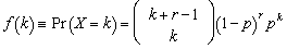 for the variables
  . In this equation, the quantity in parentheses was the binomial coefficient, which was equal to
 This quantity was also alternatively written as
  for explaining “negative binomialness’ in our regression model[2].Results from both a Poisson and a negative binomial (model residuals revealed that the district-level spatiotemporal-sampled explanatory covariate coefficient estimates were highly significant, but virtually furnished no predictive power.Inclusion of indicator variables denoting the time sequence and the district location spatial structure was then articulated with Thiessen polygons, (see Figure 2a) which also failed to reveal meaningful covariates. Further, Figure 2b implied the presence of additional noise in the data for 2010 which was attributable to an expansion of districts; thus, for this data analysis we retained the original 80 districts for space-time consistency. Next, an Autoregressive Integrated Moving Average (ARIMA) analysis of individual district time-series was generated in SAS. Given our time series district level spatiotemporal data
  where
where  was an integer index and the
  the values, an ARIMA model was built using
 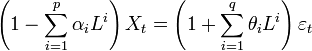 where
where  was the lag operator, the
  were the parameters of the autoregressive part of the model, the
  were the parameters of the moving average part and the
  were error terms. ARIMA models are, in theory, the most general class of models for forecasting a time series which can be stationarized by transformations such as differencing and logging[3]. The easiest way to think of ARIMA models is as fine-tuned versions of random-walk and random-trend models: the fine-tuning consists of adding lags of the differenced series and/or lags of the forecast errors to the prediction equation, as needed to remove any last traces of autocorrelation from the forecast errors[5]. In this research ehe error terms
  were generally assumed to be i.i.d. sampled from a normal distribution with zero mean:
  ~ N(0,σ2) where σ2 was the variance. Therefore, a random effects term was specified with the 80 monthly time series data (2b).This random effects specification revealed a non-constant mean across the districts that were variable which was mathematically represented a district-constant across time. This specification also represented a district-specific intercept term that was a random deviation from the overall intercept term as it was based on a draw from a normal frequency distribution. This random intercept represented the combined effect of all omitted spatiotemporal-ssampled explanatory district-level predictor covariate coefficients that caused some districts to be more prone to the malaria prevalence than other districts. Inclusion of a random intercept assumed random heterogeneity in the districts’ propensity or underlying risk of malaria prevalence that persisted throughout the entire duration of the time sequence under study. Table 1 presents the values for this random effects term, district-level for prevalence regressed on predict prevalence rates. The Poisson mean response specification was mu = exp[a + re+ LN(population)], Y ~Poisson(mu) . The mixed-model estimation results included: a = -3.1876 re ~ n(0, s2) mean re = -0.0010 s2 = 0.2513 where P(S-W) = 0.0005 and the Pseudo-R2 = 0.3103.This random effects term displayed no spatial autocorrelation and failed to closely conform to a bell-shaped curve. Its variance implied a substantial variability in the prevalence of malaria across the sampled districts in the study site. The estimated model contained considerable overdispersion (i.e., excess Poisson variability): quasi-likelihood scale = 76.5648. Figure 3 portrays scatterplots of observed versus predicted prevalence rates for selected months, and reflected the considerable amount of noise in the malaria prevalence data feature attributes as well as the random effects term accounting for about a third of the variance in the space-time series of malaria prevalence quantified. Based on the sampled district level random effects a model was then generated. As with most statistical procedures, the random effects term corresponded more closely with the data in the center of the time-series. This goodness-of-fit feature implied that although the random effects term can be used for predictive purposes, it was less effective for lengthy (e.g. > 1 year) forecasts.
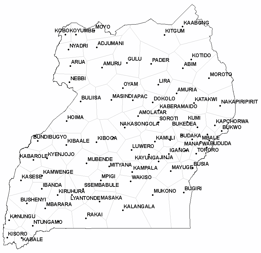 | Figure 2a. District Level Thiessen Polygons |
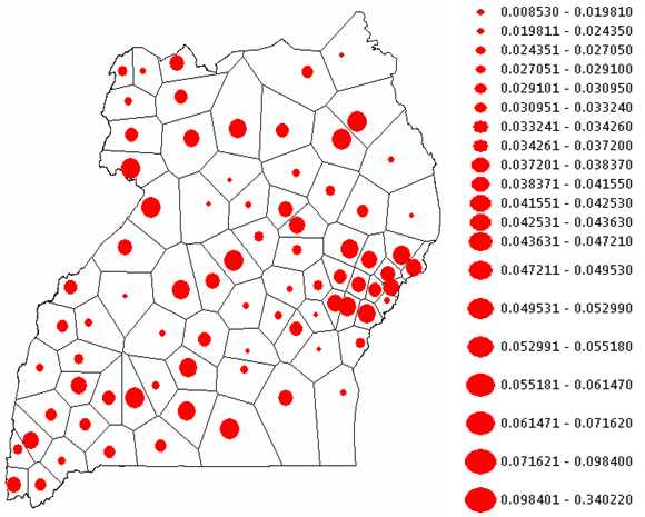 | Figure 2b. Predictive prevalence based on random effects |
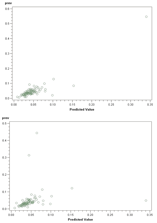 | Figure 3. Scatterplots of selected observed versus predicted district for Abimin December 2010 and Tororo 2006 |
4. Discussion and Conclusions
- Initially, in this research we constructed a Poisson regression model using spatiotemporal sampled district-level explanatory predictor covariate coefficients. The Poisson regression model constructed in this research assumed the response variable Y (i.e., prevalence) had a Poisson distribution, and assumed the logarithm of its expected value can be modelled by a linear combination of district-level parameter estimators. Unlike normal distribution, the Poisson is a natural distribution for count data[2]. However, overdispersion in our regression coefficients suggested that the Poisson model was inappropriate for differentiating the district-level covariate coefficient estimates. In this research the Poisson regression residuals indicated an inappropriate model fit due to overdispersion caused by outliners. More precisely the overdispersion implied that there was more variability around the district-level malaria model fitted values than was consistent with a Poisson formulation. We then constructed a negative binomial as a means to correct for the overdispersion. In this research the negative binomial was estimated as a generalized linear model (GLM) and as a full maximum (quasi-) likelihood model. We had to specify the distribution of the dependent variable (i.e., district-level malarial rate) in dist = negbin, as well as the link function, superscript c. By default, when we specified dist = negbin, the log link function was assumed and, thus, did not need to be further specified; however, for pedagogical purposes, we included link = log. We then wrote our model out as log (μ) = β0 + β1x1 + ... + βpxp, where μ was the log- transformed district-level prevalence count, which defined the link function. A negative binomial regression framework with a gamma distributed non- homogenous mean was then rendered which was used to attain accurate regression-based inferences from the spatiotemporal-sampled district-level explanatory predictor covariate coefficient estimates over the unbounded positive range whose sample variance exceeded the sample mean. We assumed that the dependent variable was, thereafter, no longer ill-dispersed (i.e., either under- or over- dispersed) and did not have an excessive number of zeros. In the circumstances when there is a surplus of zero measured explanatory predictor covariate coefficients in a spatiotemporal -sampled district-level malarial parameter attribute dataset, a zero-inflated negative binomial regression with a non-homogenous mean may be used for modeling count outcome variables. By so doing, excess zeros in seasonal-sampled data can be generated by a separate process from the district-level count values which can then be then modelled independently.A SAR and a spatial filter model specification was then constructed to help describe selected Gaussian and Poisson random variables rendered from the district-level malarial- related autoregressive model. When coupled with regression equations and a normal probability model, an autoregressive specification can result in a covariation term characterizing autocorrelation uncertainty components in ecological empirical datasets of field and remote-sampled malaria- related georeferenced explanatory predictor covariate coefficient estimates[1]. In this research, the SAR used a response variable, Y, as a function of nearby sampled Y district-level values[i.e., an autoregressive response (AR)], and/or the model residuals of Y as a function of nearby Y district-level sampled model covariate coefficient estimate [i.e., spatial error specification].Unfortunately, in our eigenfunction decomposition spatial filtering analyses using the district-level sampled data feature attributes, synthetic variates appeared in the numerator of Moran’s I. Thus, mean, variance and statistical distribution characterizations and descriptions of the georeferenced random variables and their interrelationships were not orthogonally derived in terms of the spatial filters. The dependency in our model was then qualitatively assessed using random effect specifications. Random effects model specifications address samples for which independent observations are selected in a highly structured rather than random way, and involve repeated measures in frequentist analyses[2]. This average, however, in this research, ignored both spatial and serial uncertainty correlation coefficients in the space-time series. A random effects model essentially works with these averages, adjusting them in accordance with the correlational structure parent space-time series, as well as their simultaneous estimation[3]. For example, in this research, the random effects model specification was achieved by fitting a distribution with as few parameter estimators as possible (e.g., a mean and a variance for a bell-shaped curve), rather than n means (i.e., fixed effects) for the n sampled district-level locational attributes. Consequently, a relationship existed between the time-series means and the random effects. This random effects specification included n indicator variables, each for a separate specific district local intercept (i.e., one local intercept was arbitrarily set to 0 to eliminate perfect multicollinearity with the global mean). Here, the local mean for district 80 was set to 0. The estimated global mean was -3.6723, the mean of the random effects term was -0.0010, and the mean of the local means was 0.4837; the sum of these three values was -3.1876, which in this research was exactly the same as the random effects global mean. The scatterplot of the random effects versus the local intercepts corresponded to a straight line with no dispersion about it.In the future, meta-analyses of spatiotemporal sampled district-level malarial indices in Uganda may employ a random-effects model to remotely account for unobserved heterogeneity among varying sentinel sites since these data feature attributes would encompass variation beyond those associated with fixed effects. For example, a random-effects linear regression approach can allow for the inclusion of various times series-dependent sentinel site explanatory predictor covariate coefficients that may explain seasonal heterogeneity in attributes associated to district-level malarial prevalence rates. A simulation study for a random- effects regression method may also perform well in the context of a meta-analysis for qualitatively assessing district-level spatiotemporal-sampled predictor covariate coefficients for robustness especially where certain factors are thought to modify larval control efficacy (e.g., seasonal rainfall production). A smoothed estimator of the within- study variances may also produce less bias in the estimated linear regression-based coefficients, thereby, rendering robust asymptotical optimized efficient estimates. Additionally, the method can provide very good power for detecting a non-zero intercept term representing overall treatment efficacy in a district-level malarial-related hyperendemic model. The model may then be also applied to the meta-analysis of continuous outcomes quantitatively derived from time-series-related seasonally dependent datasets of sentinel site-related explanatory predictor covariate coefficients. Thus, suppose that an n sampled sentinel site is chosen randomly at a selected district throughout an epidemiological district-level study site. Thereafter,Yij would be used for sampled covariate coefficient values of the jth sample site at the ith district for ascertaining statistical significance of the sentinel site sampled parameter estimators. A simple way to model the relationships of these quantities would then be
 where μ is the time series sampled district-level sentinel site explanatory predictor covariate coefficients measurement indicator values. In this model Ui would represent the specific sentinel site specific random effect. This linear hierarchical effect would then be used to measure the difference between the measured sample sites at sentinel site i and the measured values in the entire district area. The term, WI in would then be the individual sampled district-level site specific error. That is, WI would be the deviation of the j-the sampled sentimental site data from the i-th district level sampled covariate coefficients. This analyses then would be regarded as random as the selection of the sentinel sites within the district would be random even though it would be fixed quantities. Theoretically, thereafter, the sentinel site malarial –related model can be augmented by including additional spatiotemporal seasonal-sampled explanatory predictor covariate coefficients, which would then enable capturing and forecasting linear differences in sentinel sampled sites in different regional districts. For example, the variance of Yij could be adjusted to be the sum of the variances τ2 and σ2 of Ui and Wij respectively in a specific district. We can even then let
 be the average, at the ith sentietel sites, but only of those at the ith district site that are included in the random sample. Additionally, we can let
  be the "grand average". of the sentinel site data feature attributes seasonally collected in a district. Subsequently, we can then let the equation
  and
and  be respectively the sum of squares due to differences within the sentinel sites and the sum of squares due to difference between districts. Thus, it can be easily shown that
  and that
  These "expected mean squares" can then be used as the basis for estimation of the "variance components" σ2 and τ2 for seasonally quantifying time series-dependent sentinel- sampled malarial-related explanatory predictor covariate coefficients at the district and regional level.In conclusion results from both a Poisson and a negative binomial regression(i.e., a Poisson random variable with a gamma distrusted mean) revealed that the district-level seasonal-sampled explanatory predictor covariate coefficients were highly significant, but furnished virtually no predictive power. In other words, the sizes of the population denominators were sufficient to result in statistically significant relationships while the detected relationships were inconsequential. Inclusion of indicator variables denoting the time sequence and the district location spatial structure was then articulated with Thiessen polygons which also failed to reveal meaningful estimates. Unfortunately, the presence of additional noise in the data for 2010 was determined to be attributable to an expansion of districts which did not allow for forecasting the sampled district-level data employing a spatial filter algorithm. As such, the data analysis retained only the original 80 districts in the space-time consistency analyses. Thereafter, an ARIMA analysis of individual district time-series revealed a conspicuous but not very prominent first-order temporal autoregressive structure in the sampled data. As such, a random effects term was specified with the monthly time series variables. This random intercept represented the combined effect of all omitted district-specific covariate coefficients that caused districts to be more prone to the malaria prevalence than other districts. The random effects term displayed no spatial autocorrelation, and failed to closely conform to a bell-shaped curve. The variance, however, implied a substantial variability in the prevalence of malaria across districts. The estimated model contained considerable overdispersion (i.e., excess Poisson variability). The following equation was then generated to forecast the expected value of the prevalence of malaria for district: prevalence =exp[-3.1876 + (random effect)i] .The goodness- of-fit feature implied that the random effects term can be used for forecasting purposes. The model however also indicated the autoregressive residuals were less effective for forecasting purposes especially for a relatively lengthy time. Compilation of additional data can allow continual updating of the random effects term estimates, allowing rolling in new-data informed results to bolster the quality of the predictions for future time-series dependent malarial-related seasonal district-level modelling efforts.
 Notes
1Adjusted cases were calculated by rounding off prevalence*population to obtain integer counts.
References
| [1] | B.G Jacob, K.L. Arheart, D.A. Griffith, C.M. Mbogo, A.K. Githeko and J.L. Regens, ”Evaluation of environmental data for identification of Anopheles (Diptera: Culicidae) aquatic larval habitats in Kisumu and Malindi, Kenya,” Journal of Medical Entomology, Vol. 42, No. 5, 2005, pp. 751-755. |
| [2] | F.A. Haight, “Handbook of the Poisson Distribution,” Wiley Press, New York, 1967. |
| [3] | D.A. Griffith, “Spatial autocorrelation and spatial filtering: Gaining understanding through theory and scientific visualization,” Springer-Verlag, Berlin, 2003. |
| [4] | W. Gu and R.J. Novak, “Habitat-based modeling of impacts of mosquito larval interventions on entomological inoculation rates, incidence, and prevalence of malaria,” American Journal of Tropical Medicine and Hygiene, Vol. 73, 2005, pp. 546–552. |
| [5] | N.Nielsen, Een Raekke for Euler’s Konstnat,” Nyt. Tidss for Math., Vol.8B, 1897, pp.10-12. |
| [6] | J. Sondow and W. Zudilin, “Euler's Constant,  -Logarithms, and Formulas of Ramanujan and Gosper,” Ramanujan J., Vol. 12, 2006, pp. 225-244. -Logarithms, and Formulas of Ramanujan and Gosper,” Ramanujan J., Vol. 12, 2006, pp. 225-244. |
| [7] | C. de la Vallée Poussin, “Sur les valeurs moyennes de certaines fonctions arithm´etiques,” Annales de la soci´et´e scientifique de Bruxelles, Vol. 22, 1898, 84–90.. |
| [8] | W. Gosper, “Item 120,” In: M. Beeler, R.W. Gosper and Schroeppel eds., MIT Artificial Intelligence Laboratory, Memo AIM-239, Cambridge, Massachussetts, 1972, pp. 55. |