Ramesh Naidu Annavarapu1, 2
1Department of Physics, School of Physical, Chemical and Applied SciencesPondicherry University, Puducherry, 605 014, India
2Neuroscience Center, University of Helsinki, Finland, 00014, Finland
Correspondence to: Ramesh Naidu Annavarapu, Department of Physics, School of Physical, Chemical and Applied SciencesPondicherry University, Puducherry, 605 014, India.
| Email: |  |
Copyright © 2012 Scientific & Academic Publishing. All Rights Reserved.
Abstract
The different orthogonal relationship that exists in the Löwdin orthogonalizations is presented. Other orthogonalization techniques such as polar decomposition (PD), principal component analysis (PCA) and reduced singular value decomposition (SVD) can be derived from Löwdin methods. It is analytically shown that the polar decomposition is presented in the symmetric orthogonalization; principal component analysis and singular value decomposition are in the canonical orthogonalization. The canonical orthogonalization can be brought into the form of reduced SVD or vice-versa. The analytic relation between symmetric and canonical orthogonalization methods is established. The inter-relationship between symmetric orthogonalization and singular value decomposition is presented.
Keywords:
Canonical Orthogonalization, Polar Decomposition, Principal Component Analysis, Reduced Singular Value Decomposition, Symmetric Orthogonalization
Cite this paper: Ramesh Naidu Annavarapu, Singular Value Decomposition and the Centrality of Löwdin Orthogonalizations, American Journal of Computational and Applied Mathematics, Vol. 3 No. 1, 2013, pp. 33-35. doi: 10.5923/j.ajcam.20130301.06.
1. Introduction
Orthogonalization methods come in two categories, viz., sequential and democratic. The Gram-Schmidt method[1] takes the linearly independent set of vectors one-by-one and gives an orthonormal set. The democratic orthogonalization methods due to Löwdin namely the symmetric and canonical orthogonalizations handle all the given vectors simultaneously and treat them on equal footing. Löwdin orthogonalization methods[2, 3, 4] were discovered for the purpose of orthogonalizing hybrid electron orbits in quantum chemistry. A few other orthogonalization methods have been developed independently to deal with specific problems in computer science, mathematics, statistics and biology etc. A comparision of Löwdin orthogonalization schemes to other orthogonalization techniques such as polar decomposition, principal component analysis and singular value decomposition is presented. The derivation and interesting geometric properties of these two procedures are described in the references[2, 5, 6]. Applications of Löwdin methods to a variety of interdisciplinary problems have been explored in the last decade. They have applications in cognitive phenomena[7, 8], data reduction[9] and in the generation of new polynomials[10].
2. A Brief Overview of Löwdin Orthogonalization Methods
Let  be a set of m-linearly independent vectors in ann-dimensional space which can in general be a complex vector space. A general non-singular linear transformation A can transform the basis V to a new basis Z:
 | (1) |
The set  will be orthonormal if
 | (2) |
where M is a Hermitian metric matrix of the given basis V.A general solution to the orthogonalization problem is obtained using the substitution | (3) |
where B is an arbitrary unitary matrix.The specific choice  gives the symmetric orthogonalization,
 | (4) |
while  where Udiagonalizes M gives the canonical orthogonalization,
 | (5) |
These two orthogonalized basis sets have novel geometric properties[5] whileconsider the Schweinler-Wigner matrix[6] in terms of the sum of squared projections.
3. Results
3.1. Polar Decomposition
The polar decomposition[11] of a matrix  where R is a set of real numbers, can be obtained from the Löwdin’s symmetric orthogonalization. The symmetric orthonormal basis of a matrix Vis expressed as
 | (6) |
where  Now multiplying both sides of eqn. (6) from right by
  , we get
 | (7) |
This is called as polar decomposition of the matrix V.
3.2. Principal Component Analysis
Let  , then the sum of squares and cross-products (SSCP) matrix Scan be constructed using
  The SSCP matrix is the covariance matrix without subtracting the mean. The diagonal values are sums of squares and the off-diagonal values are sums of cross products. The eigenvalues and eigenvectors of the SSCP matrix Sare constructed. We have found that the eigenvalues are the same as the eigenvalues of the Gram matrix constructed using
  in the case of Löwdin orthogonalizations. The eigenvectors in the two cases are different. However, the eigenvectors of the SSCP matrix S, called as the principal components[12] of V, are the same as those obtained using the canonical orthogonalized set
  . The eigenvectors of S are ordered so that the first two principal components retain most of the variance present in the original set of vectors. We have computed the sum of the projection-squares[5] of the given vectors onto principal components[5, 13]. This gives the eigenvalues of Sand is the same as the sum of projection-squares of the original vectors on the canonical orthonormal vectors, i.e., theeigenvalues of M. For mvectors in n dimensions, we find that the principal components obtained through the principal component analysis of a square matrix V are equal to the orthonormal vectors obtained through the Löwdin’s canonical orthogonalization. Hence in the case of square matrices, the principal component analysis of the pure SSCP matrix is equivalent to the canonical orthogonalization.
3.3.Singular Value Decomposition
The singular value decomposition[14, 15, 16] of a non-singular matrix V can be obtained from the Löwdin’s canonical orthogonalization. The canonical orthogonalization of a matrix Vcan be written as | (8) |
Multiplying both sides of equation (8) from its right with d1/2, we have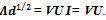 | (9) |
Now multiplying equation (9) on both sides from right with U†, we get | (10) |
This is the singular value decomposition of matrix Vand is called as reduced singular value decomposition form of the canonical orthogonalization.
3.4. Analytic Relations between Symmetric and Canonical Orthogonalizations
We can analytically obtain the relationship between symmetric and canonical orthogonalizations. If one of them is obtained from the Hermitian metric matrix, say canonical or symmetric, then the other can be obtained from the following fundamental relations.The symmetric orthonormal basis is given by | (11) |
From the equation  We have
 | (12) |
 | (13) |
This analytic relation is useful to construct the canonical orthonormal basis directly using symmetric orthonormal basis and the eigenvectors of the Hermitian metric matrix. The symmetric orthonormal basis can be obtained from the canonical orthonormal basis by multiplying both sides of equation (13) from its right with U†as shown below. | (14) |
 | (15) |
 | (16) |
3.5. Symmetric Orthogonalization in SVD
We can analytically obtain the symmetric orthogonalization[17] from the singular value decomposition. Let  with n ≥ m be a non-singular matrix. Then the singular value decomposition of Vcan be written as
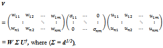 where
where  are matrices with their columns as orthonormal vectors. The columns Wj, j = 1, 2, …, m of W are called left singular vectors of V and the columns of Uj , j = 1, 2, …, ,m of U (or rows of U†) are called right singular vectors of V. And
  is square and diagonal matrix with σi’s as the singular values of V. By convention, the singular values are arranged in a descending order as σ1 ≥ σ2 ≥…≥σm ≥ 0. This form of singular value decomposition is known as reduced singular value decomposition. This reduced SVD can give the symmetric orthogonalization. Using the analytic relationship between the symmetric and canonical orthogonalizations, the symmetric orthogonalization of the matrix V can be written from the reduced SVD as follows,
 | (17) |
 | (18) |
 | (19) |
where W is the same as the canonical orthonormal basis  . The symmetric orthonormal basis
  is unique since it takes the linearly independent set of columns of V as input and gives the orthonormal columns of WU† as output. It is unique because of its two noteworthy properties[18]; one is that the symmetric bases preserve the same symmetry as the original ones and other is that the bases are least deformed from the original ones in the least-squares sense[19].
4. Discussion and Conclusions
The democratic orthogonalization procedures consider the entire lots of vectors in one go. We concentrated mainly on the democratic type because their applications have not been explored much except in the domain of quantum chemistry. We have established that the canonical orthogonalization was in fact invented independently by several people from time to time with different names such as principal component analysis and singular value decomposition. We have established their equivalence. The connections between symmetric and canonical orthogonalizations have also been established. Analytic relation between symmetric and canonical orthogonalizations methods is presented. The inter-relationship between symmetric and SVD is also shown.
ACKNOWLEDGEMENTS
The author would like to thank VipinSrivastava of University of Hyderabad for the discussions. This work is financially supported from the grant of University Grants Commission (UGC), New Delhi, India. The author would like to thank the UGC for the financial support.
References
| [1] | R. Courant and D. Hilbert, Methods of Mathematical Physics, Vol.1, 3rd Ed., IntersciencePublication, NewYork., (1953). |
| [2] | P-O. Löwdin; Ark. Mat. Astr. Fys. A., 35, (1947) pp. 9. |
| [3] | P.-O. Löwdin, Adv. Phys., 5, (1956), pp. 1. |
| [4] | J. G. Aiken, J. A. Erdos and J. A. Goldstein, Int. J. Quan. Chem., 18, (1980), pp. 1101-1108. |
| [5] | V. Srivastava, J. Phys. A: Math. Gen.,33, (2000), pp. 6219-6222. |
| [6] | H. C. Schweinler and E. P. Wigner, J.Math. Phys., 97, (1970), pp. 1693. |
| [7] | V. Srivastava and Edwards S F; PhysicaA, 276, (2000), pp. 352-358. |
| [8] | V. Srivastava, D. J. Parker, S. F. Edwards, J. Th. Biol. 253, (2008), pp. 514-517. |
| [9] | A. Ramesh Naidu and Vipin Srivastava, Int. J. Quan. Chem. 99(6), (2004), pp. 882-888. |
| [10] | VipinSrivastava and A. Ramesh Naidu, Int. J. Quan. Chem. 106, (2006), pp. 1258-1266. |
| [11] | Horn and Johnson, Matrix Analysis, Cambridge University Press, (1989). |
| [12] | I. T. Jolliffe, Principal Component Analysis, Springer-Verlag, New York, (1986). |
| [13] | R. Rojas, Neural Networks, Springer, (1996). |
| [14] | Golub, H. Gene, Van Loan, F. Charles, Matrix Computations, 3rd Ed., TheJohnHopkinsUniversity Press, (1996). |
| [15] | D. S. Watkins, Fundamentals of Matrix Computations, Wiley, NewYork, (1991), pp. 390-409. |
| [16] | G. W. Stewart, SIAM Review, Vo. 35, No. 4 (Dec., 1993), 551-566. |
| [17] | Mayer, I., 2002, Int. J. Quantum Chem., 90: 63–65. |
| [18] | Rokob, András T.; Szabados, Ágnes; Surján, Peter R., 2008, Collection of Czechoslovak Chemical Communications, 73 (6-7). pp. 937-944. |
| [19] | J. C. Slater and G. F. Koster. Phys. Rev., 94:1498, 1954. |
 Abstract
 Reference
 Full-Text PDF
 Full-text HTML