S. Kutluay, N. M. Yagmurlu
Department of Mathematics, İnönü University, 44280, Malatya, Turkey
Correspondence to: N. M. Yagmurlu, Department of Mathematics, İnönü University, 44280, Malatya, Turkey.
| Email: |  |
Copyright © 2012 Scientific & Academic Publishing. All Rights Reserved.
Abstract
In this paper, the bi-quintic B-spline base functions have been modified on a general two dimensional problem. A special form of the two dimensional problem has been considered as its application and has been solved by the Galerkin finite element method using the modified bi-quintic B-spline base functions. The computed results obtained by the present method have also been compared with the results available in the literature.
Keywords:
Galerkin Finite Element Method, Bi-quintic B-splines, Two-dimensional B-splines, Modified bi-quintic B-splines, Two-dimensional Poisson Equation
Cite this paper: S. Kutluay, N. M. Yagmurlu, Derivation of the Modified Bi-quintic B-spline Base Functions: An Application to Poisson Equation, American Journal of Computational and Applied Mathematics, Vol. 3 No. 1, 2013, pp. 26-32. doi: 10.5923/j.ajcam.20130301.05.
MSC classification: 65N30, 65N30, 65D07, 74S05
1. Introduction
The finite element method is a widely used method for solving both ordinary and partial differential equations. For a long time, the finite element method has been applied by many researchers to physics, solid and fluid mechanics, engineering, medicine, and so on[1]-[9]. The main idea behind the finite element method is to divide the whole region of the given problem into an equivalent system of finite elements with associated nodes and to choose the most appropriate element type to model most closely the actual physical behavior. Thus, by means of the finite element method, a huge problem is converted into many solvable small problems. Those elements must be made small enough to give usable results and yet large enough to reduce computational effort[3].B-spline finite element method has been previously and widely used to obtain very accurate solutions for partial differential equations in one dimensional problem[2]-[8], [10]-[15]. Nevertheless, developments in computational techniques and computer technology have shown that the method can also be effectively used to obtain accurate approximate solutions for two-dimensional problems. In this paper, the bi-quintic B-splines on the boundary of the model problem have been modified and then they have been used to solve a typical two--dimensional problem. For two-dimensional problems, there are some works in the literature.[2, 7, 9, 16].In this study, we have used bi-quintic B-splines which are only modified on the boundary of the problem as basis functions and rectangles as element shapes for a two-dimensional problem. The modified bi-quintic B-spline functions have been constructed for two dimensional problems and applied to a typical two-dimensional problem of the form . First of all, we try a bi-quintic B-spline function of the form
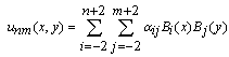 as an approximation solution to this type of equations. In order to find an approximate solution in the above form to the considered problem by the Galerkin method, first of all we have to redefine the B-spline basis functions into a new set of functions, namely modified bi-quintic B-spline functions. This redefining process was successfully applied to cubic B-spline functions to obtain modified bi-cubic B-spline functions[2]. The newly obtained set of modified functions is identically zero on the boundary of the given problem. It should be pointed out that this process is necessary, since B-spline basis functions
  in the
  -direction and the B-spline basis functions
 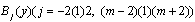 in the
  -direction are not zero on the boundary of the given problem. After the redefining process of the basis functions, we can now try the modified bi-quintic B-spline functions of the form
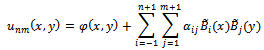 as its approximate solution, where
  and
and  are quintic B-splines modified only on the boundary in the
  and
and  - directions, respectively. Since all of the modified quintic B-splines are zero on the boundary of the given problem, non-homogenous boundary conditions are satisfied by the term
  .
. | Figure 1. The bi-quintic B-spline B₃₃ centred on (3,3) covering 36 finite elements of side 1 |
2. Derivation of the Modified Bi-Quintic B-splines
2.1. Bi-quintic B-spline Element
Suppose that a rectangular grid is subdivided into a number of uniform rectangular finite elements of sides  and
and  by the knots
  where
where 
 . An approximation
  with quintic B-spline functions to
  is of the form
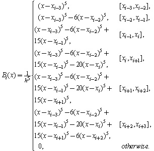
 can easily be found by replacing
  with
with  and
and  with
with  Fig.1 depicts a region where
  , so that it is divided into finite elements by the integer knots
  , and a single bi-quintic B-spline
  which peaks on the point
  and also covers a total of
  square elements. When the entire set of bi-quintic splines
  , each of which peaks on a knot
 , where
 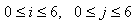 are added to this figure, a total of
  splines cover each finite element[8].
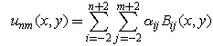 | (1) |
where are the amplitudes of bi-quintic B-splines
  given by
 | (2) |
and  is defined as[11]
2.2. A Modified Two-dimensional Quintic B-spline Element
To show how to modify bi-quintic splines on the boundary, we consider the two-dimensional general linear problem given in the form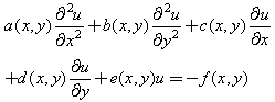 | (3) |
subject to boundary conditions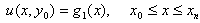 | (4) |
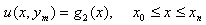 | (5) |
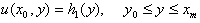 | (6) |
 | (7) |
where  and
and  ,
,  are given functions,
  is a rectangular region in
  with boundary
  .Now, it is supposed that both the
  -space variable domain and
  -space variable domain of the system (3)-(7) are divided into
  and
and  sub-intervals, respectively, by the set of
  distinct grid points
  and
and  distinct grid points
  such that
 .Since we use quintic B-splines, a quintic B-spline covers six consecutive elements, we add ten additional grid points
  in the
  -direction and ten additional grid points
  ,
, 
 in the
  -direction such that
 To obtain an approximate solution in the form of Eq. (1) to the model problem given by Eqs.(3)-(7) with the Galerkin method, we do need to redefine the basis functions into a new set of basis functions which all vanish on
  . The redefining process of the basis functions is done in the following three steps.Step1. The approximate solution
  given by Eq. (1) can also be written as[2]
 | (8) |
where | (9) |
Allowing the approximate solution  given by Eq. (8) to satisfy the boundary conditions (6) and (7) and eliminating
  and
and  from the resulting equations, we obtain
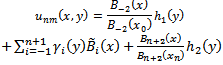 | (10) |
where | (11) |
 | (12) |
 | (13) |
Step 2. By evaluating the expression  given by Eq. (9) at
  and
and  and eliminating
  and
and  from the resulting equations, we obtain the following expression for
  :
: | (14) |
where | (15) |
 | (16) |
 | (17) |
Step 3. Finally, substituting  in Eq. (14) into Eq. (10) and allowing the resulting equation to satisfy the boundary conditions (4) and (5), we obtain
  | (18) |
where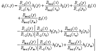 | (19) |
Applying exactly the same above steps to the approximate solution (1) to the problem given by Eqs. (3)-(7) again, but now writing the approximate solution as[2] | (20) |
where | (21) |
we obtain | (22) |
Where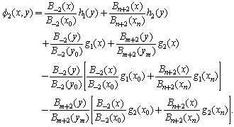 | (23) |
By taking the average of Eq. (19) and Eq. (23), we finally obtain the general approximation 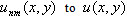 of the form
 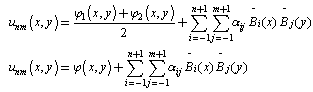 | (24) |
where the new set of basis functions are  for
for  , which all vanish on
  and
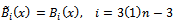
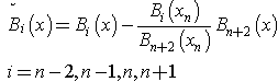
and  given in Eq. (24) satisfies the boundary conditions given by Eqs. (4) - (7). For simplicity, the modified quintic B-splines are shown in Fig.2 for only 4 elements.
 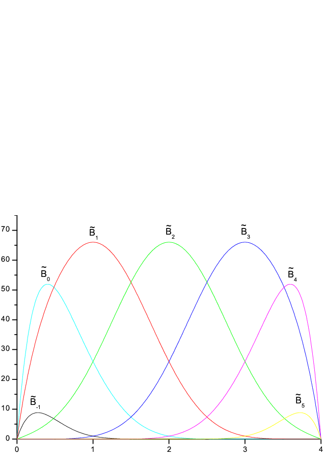 | Figure 2. Modified B-spline functions 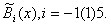 |
3. Numerical Example
There are some researches about two-dimensional Poisson equation in the literature. Wu and Zhang[7] have obtained numerical solutions of Dirichlet problem for two-dimensional Poisson equation using the Galerkin quartic B-spline finite element method. Schaerer et al.[17] have presented Multilevel Schwarz Shooting method for the numerical solution of the Poisson equation using a five point finite difference molecule, and subject to Dirichlet boundary conditions, which arises in two dimensional incompressible flow simulations. Ahmed and Monaquel[18] have developed multi-grid method with compact finite difference method of 9-point sixth order for two-dimensional Poisson equation and showed the efficiency of the method with numerical solutions.In this section, we have applied the Galerkin method using the modified bi-quintic B-spline basis functions to obtain the numerical solutions of the two dimensional Poisson problem given as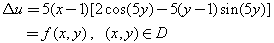
 where
where  .The exact solution of this problem is
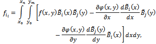
 To apply the Galerkin method with bi-quintic B-splines, we first need to find the weak formulation of the problem. Its weak form is given by the integral equation
 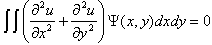 | (25) |
where  is the weight function taken as modified bi-quintic B-spline functions. Using the Green Theorem and the values of the modified bi-quintic B-spline functions on the boundary conditions, we obtain the weak form of the problem as
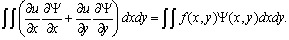 | (26) |
For the sake of simplicity, we divide the region  into
into  elements and show the procedure in detail. Thus, we have 16 squares with sides of
  , and
, and  . We use the following numeration of the region
  with
with  elements in the following processes.
 Since each part of a quintic B-spline should be multiplied by the same coefficient to satisfy the continuity condition, the modified quintic B-splines
  and
and  are multiplied by local coefficients
  and
and 
 respectively. Therefore, we have total
  global coefficients to be computed. The global coefficients and their corresponding local coefficients are determined as
 Thus, we obtain the approximations for each element by writing the linear combination of
  and
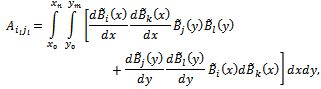
and  lying on the related element in Eq. (26).By applying the Galerkin method with

 and
and  as basis functions and with an approximation
  given by Eq.(26) to the model problem, in a similar way given in Ref.[2], we get the following algebraic system:
  where
where
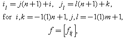
 and
and  is the coefficient vector to be computed.Assembling all contributions from all elements, we reach the global combined matrix. Since the modified bi-quintic B-splines have been altered so as to meet the boundary conditions beforehand, the resulting equations are solved without imposing the boundary conditions at the end of the element assembly process. By solving the system of equations obtained in the global combined matrix, we evaluate the values of global variables
  .Table 1 displays the obtained numerical and exact solutions of the problem with those given in Ref.[7]. It is clearly seen that the obtained numerical solutions are in very good agreement with exact ones. They are also much better than those given in Ref.[7] using quartic B-spline finite element and finite difference methods. To show how good and accurate the numerical solutions of the problem, a comparison of the obtained numerical and exact solutions at some different points are displayed in Table 2.
| Table 1. Comparison of the numerical solutions obtained by the present method with results from Ref. [7] and the exact solution at some points |
| | Present | | [7] | | | | Quintic | | Quartic | Finite Difference | | Exact | | (x,y) | (4×4) | (10×10) | | | | | | | (0.25,0.25) | 0.533970 | 0.533803 | | 0.523514 | 0.543869 | | 0.533804 | | (0.25,0.50) | 0.224352 | 0.224426 | | 0.229845 | 0.220623 | | 0.224400 | | (0.25,0.75) | -0.107419 | -0.107167 | | -0.098704 | -0.117514 | | -0.107168 | | (0.50,0.25) | 0.355980 | 0.355869 | | 0.345257 | 0.364192 | | 0.355869 | | (0.50,0.50) | 0.149568 | 0.149618 | | 0.152811 | 0.146201 | | 0.149618 | | (0.50,0.75) | -0.071613 | -0.071445 | | -0.064679 | -0.080613 | | -0.071445 | | (0.75,0.25) | 0.177990 | 0.177935 | | 0.173169 | 0.182276 | | 0.177935 | | (0.75,0.50) | 0.074784 | 0.074809 | | 0.076689 | 0.072922 | | 0.074809 | | (0.75,0.75) | -0.035806 | -0.035722 | | -0.032649 | -0.040688 | | -0.035723 |
|
|
| Table 2. Comparison of the numerical solutions obtained by the present method with a partition of 4×4=16 and 10×10=100 elements with exact ones at some points |
| | | Present | Exact | | (x,y) | (4×4) | (10×10) | | | (0.1,0.1) | 0.388262 | 0.388335 | 0.388335 | | (0.2,0.2) | 0.538588 | 0.538542 | 0.538541 | | (0.3,0.3) | 0.488891 | 0.488773 | 0.488773 | | (0.4,0.4) | 0.327186 | 0.327347 | 0.327347 | | (0.5,0.5) | 0.149568 | 0.149618 | 0.149618 | | (0.6,0.6) | 0.022734 | 0.022579 | 0.022579 | | (0.7,0.7) | -0.031608 | -0.031571 | -0.031571 | | (0.8,0.8) | -0.030308 | -0.030272 | -0.030272 | | (0.9,0.9) | -0.009757 | -0.009775 | -0.009775 | |
| (0.0,1.0) | 0.000000 | 0.000000 | 0.000000 | | (0.1,0.9) | -0.087821 | -0.087978 | -0.087978 | | (0.2,0.8) | -0.121231 | -0.121089 | -0.121088 | | (0.3,0.7) | -0.073754 | -0.073665 | -0.073665 | | (0.4,0.6) | 0.034100 | 0.033868 | 0.033869 | | (0.6,0.4) | 0.218123 | 0.218231 | 0.218231 | | (0.7,0.3) | 0.209524 | 0.209474 | 0.209474 | | (0.8,0.2) | 0.134648 | 0.134636 | 0.134635 | | (0.9,0.1) | 0.043140 | 0.043148 | 0.043148 | | (1.0,0.0) | 0.000000 | 0.000000 | 0.000000 |
|
|
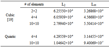
Table 3. The error norms L₂ and L∞ of the model problem for various numbers of elements and B-spline base functions
 |
| |
|
In order to measure how good the numerical solutions obtained by the Galerkin Finite Element Method with the modified bi-quintic B-spline basis functions, the error norms  and
and  defined as
  are computed and given in Table 3. Here
  is the number of inner points,
  and
and  are the exact and approximate solutions at the point
  , respectively. The error norms
  and
and  are computed by taking the values
  and
and  at
at  points obtained by dividing the region
  into equal elements in the directions
  and
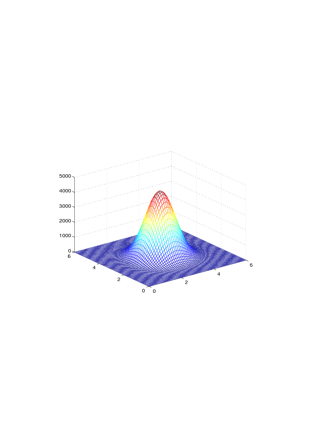
and  . As seen from Table 3, the approximate solution becomes better as the number of elements increase. Moreover, in order to demonstrate how good the numerical solutions obtained by the present method exhibit the correct physical characteristic of the problem, we also give the graphs in Figs. 3, 4 and 5 which illustrate the exact and numerical solutions with
  and
and  partitions of the model problem, respectively. It is clearly seen from the figures that both graphs are nearly indistinguishable since both solutions are in very good agreement with each other.
 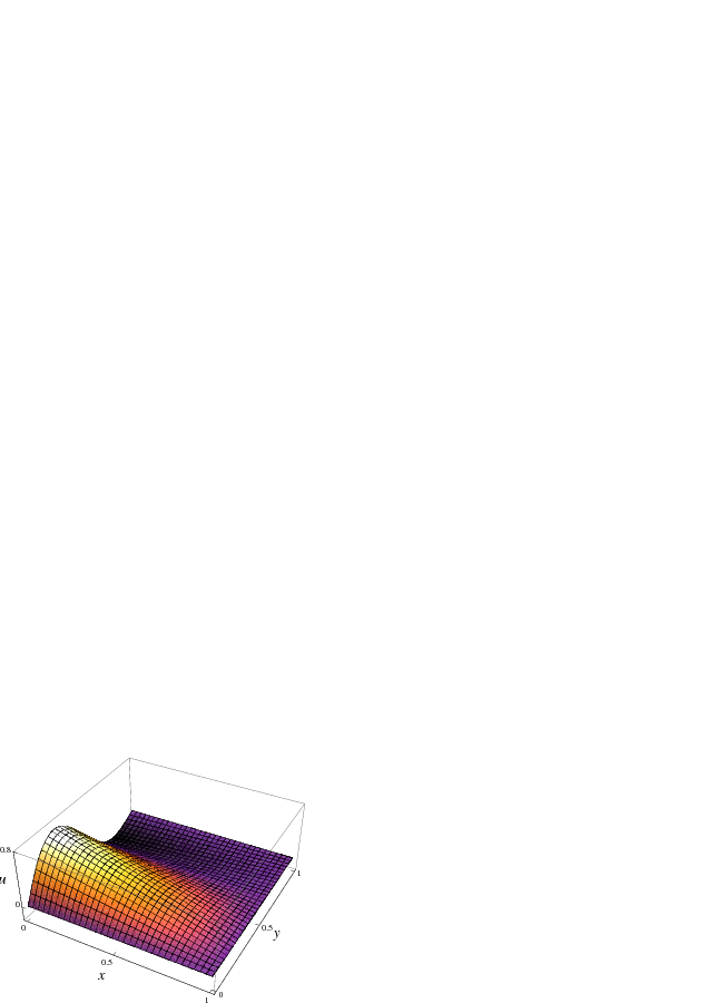 | Figure 3. Exact solution |
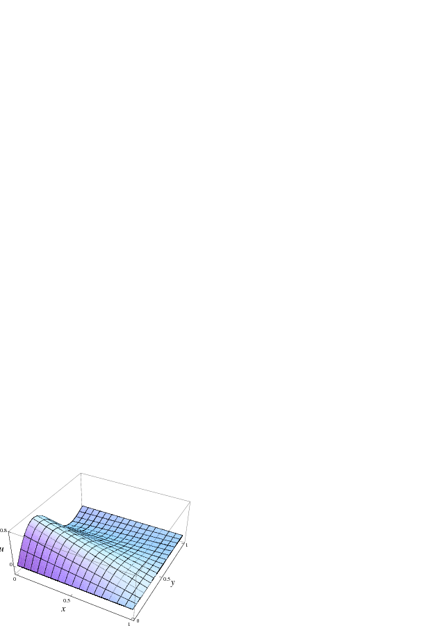 | Figure 4. Numerical solution with 16 elements partitions |
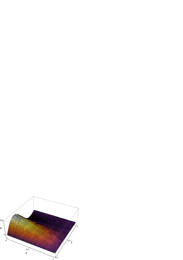 | Figure 5. Numerical solution with 100 elements partitions |
4. Conclusions
In this paper, the modified bi-quintic B-spline finite element method is proposed and successfully applied to two dimensional Poisson problem to obtain its numerical solutions. The agreement between our numerical results and the exact ones is satisfactorily good. The obtained numerical results showed that the modified bi-quintic B-spline finite element method is remarkably a successful numerical technique. In conclusion, this method with a different choice of B-spline basis functions and element numbers can also be applied to more general non-linear partial differential equations arising in physics and mathematics and resulting in both two dimensional and coupled two dimensional equations.
References
| [1] | J. N. Reddy, An introduction to the finite element method, McGraw-Hill International Editions, third ed., New York, 2006. |
| [2] | K. N. S. Kasi Viswanadham, S.R. Koneru, Finite element method for one-dimensional and two-dimensional time dependent problems with B-splines, Comput. Methods Appl. Mech. Engrg. 108, (1993) 201-222. |
| [3] | D. L. Logan, A First Course in the Finite Element Method, Thomson Learning, part of the Thomson Corporation, New York, 2007. |
| [4] | M. A. Bhatti, Fundamental Finite Element Analysis and Applications: with Mathematica and Matlab Computations, John Wiley & Sons, Inc., New York, 2005. |
| [5] | J.N. Reddy, An introduction to Nonlinear Finite Element Analysis, Oxford University Press, New York, 2008. |
| [6] | E. G. Thompson, Introduction To The Finite Element Method, Theory, Programming, and Applications, John Wiley Sons, Inc., USA, 2005. |
| [7] | J. Wu and X. Zhang, Finite Element Method by Using Quartic B-Splines, Numerical Methods for Partial Differential Equations, 10 (2011) 81-828 |
| [8] | L. R. T. Gardner and G. A. Gardner, A two dimensional bi-cubic B-spline finite element: used in a study of MHD-duct flow, Comput. Methods Appl. Mech. Engrg. 124 (1995) 365-375. |
| [9] | O. C. Zienkiewicz, The finite element method, McGraw-Hill, London, 1977. |
| [10] | S. Kutluay, A. Esen, I.Dağ , Numerical solutions of the Burgers equation by the least-squares quadratic B-spline finite element method, J Comput Appl Math 167 (2004) 21-33. |
| [11] | P. M. Prenter, Splines and variational methods, Wiles New York, 1975. |
| [12] | H. Bateman, Some recent researcher on the motion of fluids, Mon. Weather Rev. 43 (1915) 163-170. |
| [13] | J. M. Burger, A mathematical model illustrating the theory of turbulence, Advances in Applied Mechanics I, Academic Press, New York, (1948) 171-19. |
| [14] | J. D. Cole, On A Quasi Linear Parabolic Equation Occurring in Aerodynamics, Quart. Appl. Math. 9 (1951) 225-236. |
| [15] | P. Jamet and R. Bonnoret, Numerical solution of compressible flow by finite element method which flows the free boundary and the interfaces, J. Comput. Phys. 18 (1975) 21-45. |
| [16] | RC.Mittal and RK. Jain, B-splines methods with redefined basis functions for solving fourth order parabolic partial differential equations, Applied Mathematics and Computation, Vol.217, 2011, No.23,9741-9755. |
| [17] | C. E. Schaerer, E. Kaszkurewicz and N. Mangiavacchi, A multilevel Schwarz shooting method for the solution of the Poisson equation two dimensional incompressible flow simulations, Appl. Math. and Comput., 153 (2004) 803--831. |
| [18] | B. S. Ahmed and S. J. Monaquel, Multigrid Method for Solving 2D-Poisson Equation with Sixth Order Finite Difference Method, International Mathematical Forum, Vol.6, 2011,no.55,2729-2736. |
| [19] | N. M. Yagmurlu, Numerical Solutions of 2-Dimensional Partial Differential Equations with B-spline Finite Element Methods, Ph.D. Thesis, İnönü University, Malatya (Turkey), 2011 |
 Abstract
 Reference
 Full-Text PDF
 Full-text HTML