-
Paper Information
- Next Paper
- Previous Paper
- Paper Submission
-
Journal Information
- About This Journal
- Editorial Board
- Current Issue
- Archive
- Author Guidelines
- Contact Us
American Journal of Computational and Applied Mathematics
p-ISSN: 2165-8935 e-ISSN: 2165-8943
2013; 3(1): 13-22
doi:10.5923/j.ajcam.20130301.03
Iteratively Regularized Gradient Method for Determination of Source Terms in a Linear Parabolic Problem
 Abstract
 Reference
 Full-Text PDF
 Full-text HTML
Arzu Erdem
Kocaeli University, Faculty of Arts and Sciences, Department of Mathematics, Umuttepe Campus, 41380, Kocaeli, Turkey
Correspondence to: Arzu Erdem, Kocaeli University, Faculty of Arts and Sciences, Department of Mathematics, Umuttepe Campus, 41380, Kocaeli, Turkey.
| Email: |  |
Copyright © 2012 Scientific & Academic Publishing. All Rights Reserved.
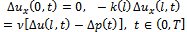
This paper investigates a numerical computation for determination of source terms in a linear parabolic problem. The source term  is defined in the linear parabolic equation
  and Robin boundary condition
  from the measured final data and the measurement of the temperature in a subregion. We demonstrate how to compute Fréchet derivative of Tikhonov functional based on the solution of the adjoint problem. Lipschitz continuity of the gradient is proved. Iteratively regularized gradient method is applied for numerical solution of the problem. We conclude with several numerical tests by using the theoretical results.
Keywords: Inverse Coefficient Source Problem, Parabolic Equation, Adjoint Problem, FrÉChet Derivative, Lipschitz Continuity
Cite this paper: Arzu Erdem, Iteratively Regularized Gradient Method for Determination of Source Terms in a Linear Parabolic Problem, American Journal of Computational and Applied Mathematics, Vol. 3 No. 1, 2013, pp. 13-22. doi: 10.5923/j.ajcam.20130301.03.
Article Outline
1. Introduction
- In describing the heat conduction in a material occupying a domain
 , the temperature distribution
  is modeled by
  | (1) |
 | (2) |
 | (3) |
 denotes internal heat source,
  is spatial varying heat conductivity,
  is an initial condition and
  denotes the convection between conducting body and the ambient environment. If one cannot measure the pair
  directly, one can try to determine
  from the final state observation of
 | (4) |
 over subregion
 ,
,  | (5) |
 has been investigated in[16,17]. To solve the inverse source problem one can use explicit and implicit methods[5,6,15,19,25]. Explicit methods provide analytical solutions to the inverse source problem directly from measured data. Explicit methods are limited to simple medium geometries with spatially non-varying optical parameters . For more complex geometries and heterogeneous media no explicit methods are available and implicit methods need to be employed. Implicit methods for solving the inverse source problem iteratively utilize a solution of a forward model to provide predicted measurement data. An update of an initial source distribution is sought by minimizing a functional that describes the goodness of a fit between the predicted and experimental data. Our approach is based on quasisolution approach. We also introduce an adjoint problem. Adjoint problem technique computes the gradient of the objective function. The concept of the adjoint problem technique can also be applied to similar inverse problems[10,13,14] or sensitivity analysis where the derivative of an error function is sought. A distinct advantage of using that technique is relatively simple numerical implementation and the resulting low computational costs. In view of quasisolution approach,this inverse problem can be formulated as minimization problem for the objective function[27]. In most cases for the numerical solution of this minimization problem gradient methods are used[4]. For this aim, in many applications various gradient formulas are either derived empirically, or computed numerically[21]. Although an empirical gradient formula has been employed with regularization algorithm,there was no mathematical framework for this formula. At the same time, we need to estimate the iteration parameter for any gradient method. Choice of the iteration parameter defines various gradient methods,although in many situation estimations of this parameter is a difficult problem. However,in the case of Lipschitz continuity of the gradient of the objective function the parameter can be estimated via the Lipschitz constant,which subsequently improves convergence properties of the iteration process [29]. In this paper we shall show how the adjoint problem technique can be readily utilized in proving Fréchet differentiability of the objective function. This has been hinted at in previous treatments[16]. Here we extend the objective function including the regularization parameter. Then we show how the Fréchet differentiability result is readily extended to examine Lipschitz continuity properties of the operator. Finally, we shall illustrate the application of our technique. The paper is outlined as follows. We summarize the basic notation and definition of regularized objective function in Section 2. Fréchet differentiability of the objective function results proven in Section 3 gives a unique regularized solution of the inverse problem. Iteratively regularized gradient method is proposed to obtain the numerical solution and some numerical examples are presented in Section 4 .
 2. Regularization Method
- Let us denote by
 the set of admissible unknown sources
  and
and  . The scalar product in
  is defined as follows:
 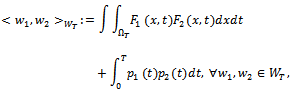 where
where  We also assume that
 . We denote the unique solution of problem (3) by
 , corresponding to this source term. The direct problem could be to predict the evolution of the described system from knowledge of
 . We denote by
  the set of measured output data
  and
and  the set of measured output data
  and set
 . Hence the inverse problem (3)-(4) can be formulated in the following operator form
  | (6) |
 is defined to be the input-output mapping. We can give the definition of scalar product in
  as similar as in
  :
:  There is a fundamental difference between the direct and the inverse problems. In all cases, the inverse problem is ill-posed or improperly posed in the sense of Hadamard, while the direct problem is well-posed. A mathematical model for a physical problem is called as well-posed in the sense that it has the following three properties: There exists a solution of the problem (existence). There is at most one solution of the problem (uniqueness). The solution depends continuously on the data (stability). When the operator
  is a bounded, linear and injective between Hilbert spaces
  and
and , and
, and  , the existence and uniqueness of the mapping is clear. If the desired output data
  and
and  are not attainable, one tries to get approximation
  and
and  as close as possible
  and
and  , respectively. Then the function
 will be defined to be the final state noisy output data and the noisy data over the subregion. For the analysis of the approximation quality of the regularized solutions, we require that a bound on the data noise
  The problem to solve (3)-(4) with noise data
  may be equivalently reformulated as finding the minimum of the functional which has been given in[16] for the only final state output data :
  On the other hand, in the case where
  is given, the inverse problem of determining
  from the observation
  , can be transformed to a Fredholm equation of the second kind, where there might exist a non-trivial solution which implies the non-uniqueness for such an inverse problem. Of course, the solution to this minimization problem again does not depend continuously on the data. One possibility to restore stability is to add the data over the subregion and a penalty term to the functional involving the norm of
 :
:  | (7) |
 is called regularization parameter. A regularized solution
  is defined by
  Regularization methods replace an ill-posed problem by a family of well-posed problems, their solution, called regularized solutions, are used as approximations to the desired solution of the inverse problem. These methods always involve some parameter measuring the closeness of the regularized and the original (unregularized) inverse problem, rules (and algorithms) for the choice of these regularization parameters as well as convergence properties of the regularized solutions are central points in the theory of these methods, since only they allow to finally and the right balance between stability and accuracy.
 3. Properties of Regularization Method
- This section contains the main results of this paper. In the forthcoming theorem, we prove that the the functional (7) is Fréchet differentiable and provide the explicit form of the derivative. Let us give some preparations. Definition 3.1. Let X, Y be normed spaces, and let U be an open subset of X. A mapping
 is called Fréchet differentiable at
  if there exists a bounded linear operator
  such that
 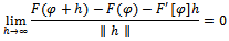 The proof of the following lemma can be found in[16]. Lemma 3.2. Let
  be two solutions of direct problem (3) corresponding to admissible sources
 The following equality holds:
 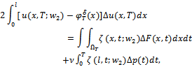 | (8) |
 ,
,  ,
, 
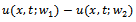 is the solution of the following sensitivity problem
  | (9) |
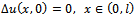 | (10) |
 | (11) |
 is the solution of the backward parabolic problem:
 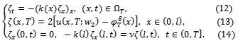 Lemma 3.3. Let
  be two solutions of direct problem (3) corresponding to admissible sources
 The following equality holds:
 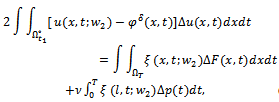 | (15) |
 is the solution of the backward parabolic problem:
 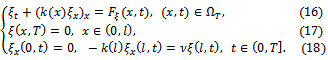 with the following discontinuous right-hand side
 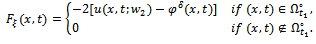 Proof. We start by replacing the left hand side of equality (15) with the right hand side of problem (18):
  We use integration by parts
 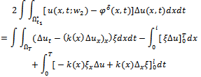 and employ initial and boundary conditions of problems (11) and (18) we conclude the proof of the lemma. The following Lemma gives computation of the first variation of the functional (7). Lemma 3.4. Let us denote by
 .
.  the first variation of the functional (7) is given by
 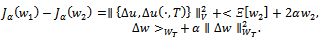 | (19) |
 Employing some add and subtract tricks, we get
  Finally, this with the integral identities (8) and (15) leads to
  Lemma 3.5. There exists a constant
  such that
  | (20) |
 is solution of the parabolic problem (11). Proof. One can have this result due to Lemma 3.2 of[16]. Lemma 3.6. There exists a constant
  such that
 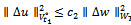 | (21) |
 is solution of the parabolic problem (11). Proof. Due to the energy equality of the parabolic problem (11), we write
 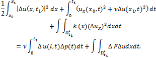 Applying Cauchy
  inequality to the right hand side of the above equality we obtain
 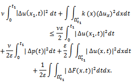 | (22) |
 we have
  | (23) |
 , we get the following estimate:
  and satisfies
  | (24) |
 . In this case requiring
  we obtain the bound
  . Further from the requirement
  we have the second bound
  . Thus assuming for the parameter
 Taking into account (23) and (24)
  where
where  Theorem 3.7. Assume that
 and
and  is the solution of the parabolic problem (11) corresponding to admissible source
 . Then, the functional (7) is Fréchet differentiable, with Fréchet differential:
  | (25) |

 Proof. We take the two sources
  ,
,  instead of
  in (19)
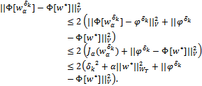
  Using the estimates in lemma 5 and lemma 6 , we have
  Then due to Definition 1 we conclude Fréchet derivative of the functional (7)
  Theorem 3.8. If conditions of Theorem 7 hold, then the functional (7) has a unique solution
  in
in  for
for  . This minimum is given by the solution of the following equation:
  Moreover
  Proof. Assume that
  minimizes the functional (7). The choice
  implies by (25) that
  To show that
  defined by the solution of above equation minimizes the functional (7), note that for all
  the function
  is a polynomial of degree 2 with
  and
and  Hence
Hence  with the equality only
  implies that
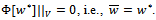
  is a minimization of the functional (7). Due to the convexity of the functional (7), we obtain the uniqueness of the solution. Since the functional (7) attains its minimum at
 and
and  , we have
  which implies
  | (26) |
 converges towards a solution of (6) in a set-valued sense with and
 . Theorem 3.9. Let
  be a weakly closed set and
  be the exact solution of (6) in
  . If
. If  is injective and
 , then
  converges to
  as
as  tends to zero. Proof. Let us assume the contrary. Then there exist an
  and a sequence
  such that
 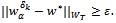 Since the functional (7) attains its minimum at
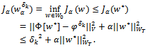 | (27) |
 | (28) |
 , such that
  . Then we obtain
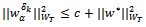 . Further, using the weak compactness of a ball in Hilbert space we conclude that
  converges weakly to
  , since
  is a weakly closed subset. Together with lower semicontinuity of the norm and inequality (28)
 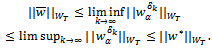 | (29) |
 By limit transition as
 , we conclude
 Due to the weak converges we obtain
  . This contradiction proves the theorem.
4. Identification Process and Computational Results
- Another idea is to minimize the functional (7) by gradient method. This leads to the recursion formula of Conjugate Gradient Method
 | (30) |
 is the search step size,
  is the direction of descent,
  is the iteration parameter. The direction of descent
  is given as
  | (31) |
 can be found as Polak-Ribiere or Fletcher -Reeves[1,7,11] . In the Polak-Ribiere version of the conjugation coefficient
  can be obtained from the following expression:
 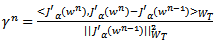 | (32) |
 is given by the following expression:
 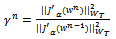 | (33) |

 | (34) |
 defined by (6) than just continuity. In particular to generate an affine approximation to
  required to be Fréchet differentiable that we have already obtained in the previous section. To obtain high-order convergence properties of the numerical method this Fréchet derivative must also be Lipschitz continuous. For the next results we refer to[16,17] Theorem 4.1. If
  and
and  are the solutions of problems (3) and (14), respectively then
  and the following estimate holds:
  | (35) |
 , Then
  implies
  The proof of monotonicity of the sequence
  is given by Corollary 4.1 in[16]. Theorem 4.3. The sequence
  is a monotone decreasing sequence. Moreover;
  Since an expression for the gradient
  of the functional (7) is explicitly available, and easily obtained by solving the adjoint problem (14), the gradient can be readily implemented. Gradient algorithm[22] applied to the optimization problem takes the form Step 1 Choose
 , and set
 . Step 2 Solve the direct problem (3) with
 and determine the residuals
  Step 3 Solve the adjoint problems (14) and (18) Step 4 Compute the gradient
  with (25). Step 5 Update the conjugation coefficient
  from (32) or (33) and then the direction descent
  from (31). Step 6 By setting
  solve the sensitivity problem (11) to obtain
  and
and  on subregion . Step 7 Compute the step size
  form (34). Step 8 Update
  from (30). Step 9 Stop computing if the stopping criterion
  is satisfied. Otherwise set
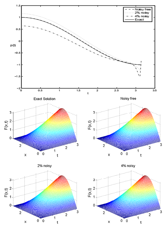
  and go to Step 2. Now, we perform some numerical experiments using the above algorithm. Example 4.4. In the first numerical experiment we take
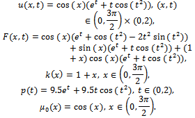 The final state observation and the observation over the subregion
  are given by
  It is easy to check that
  satisfies the problem (3) for
 . The noisy data
  and
and  are generated as follows:
  where
where  is the noisy level and
  is generated by MATLAB function
 . The exact solutions
  and
and  together with the numerical solutions for various values of the noisy level
  are shown in Figure 1. Due to the discrepancy principle we use the stopping criteria as
  where the value of the tolerance
 , for noisy free data
  and the regularization parameter
  Example 4.5. In the second numerical experiment we take
 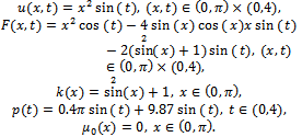 The final state observation and the observation over the subregion
 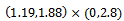 are given by
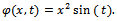
 satisfies the problem (3) for
 The exact solutions
  and
and  together with the numerical solutions for various values of the noisy level
  are presented in Figure 2. The stopping criteria is
  for noisy free data and the regularization parameter
 | Figure 1. Results obtained by conjugate gradient method for Example 4.4 |
 | Figure 2. Exact solution and and numerical experiment of  and and  for various amounts of noise p ={1, 2}% for Example 4.5 for various amounts of noise p ={1, 2}% for Example 4.5 |
 and
and  when an analytical solution for the problem (3) is not available:
 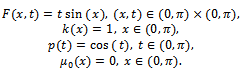 The final state observation and the observation over the subregion
  are computed by numerically for
 . The exact solutions
  and
and  together with the numerical solutions for various values of the noisy level
  are presented in Figure 3. The stopping criteria is
  for noisy free data and the regularization parameter
 .
.  | Figure 3. Exact solution and construction of  and and  for various amounts of noise p ={2, 4}% for Example 4.6 for various amounts of noise p ={2, 4}% for Example 4.6 |
|
 and
and  with various noisy level for Example4.4, Example4.5 and Example4.6
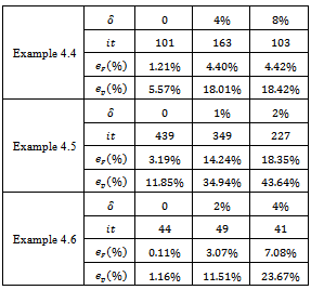
 and
and . Here we use the symbol it as the stopping iteration numbers,
  and
and  as the percentage error in
  and
and , respectively where
  and
and  are approximate value of
  and
and .
.