Chigbogu G. Ozoegwu, Sam Omenyi, Sunday M. Ofochebe
Department of Mechanical Engineering, Nnamdi Azikiwe University, Awka, PMB 5025, Nigeria
Correspondence to: Chigbogu G. Ozoegwu, Department of Mechanical Engineering, Nnamdi Azikiwe University, Awka, PMB 5025, Nigeria.
| Email: |  |
Copyright © 2012 Scientific & Academic Publishing. All Rights Reserved.
Abstract
People working in workshop have observed that there exist magic spindle speeds for any milling tool-workpiece combination at which optimal depth of cuts are allowed. Some of them have tried to unravel these magic spindle speeds experimentally. This is a very time consuming, costly and inaccurate optimization procedure thus the purpose of this work is to outline an analytical solution to not only the problem of finding the magic spindle speeds but also problem of separating the whole of stable operations from the unstable ones. Slotting three tooth end miller was studied using the method of time finite element analysis (TFEA) and validated using the result of time domain stability analysis stemming from MATLAB dde23 solution of the milling equation. It is seen for the studied system that though accuracy improves with increase in number of time elements used, only marginal gain in accuracy could be achieved by increase in number of elements above ten finite time elements. In other words close agreement exists between the two approaches (TFEA and MATLAB dde23) when the number of time elements is high enough. Fourteen time elements were used to generate a working chart for the studied system. The stability chart is seen to exhibit milling stability characteristics of magic spindle speeds already known by workshop practitioners. The major implication of this study becomes that time loss that is occasioned by experimental trial and error method of determining the productive spindle speeds is avoided.
Keywords:
Time Finite Elements, Regenerative Effects, Stability, Matlab dde23, Optimal Depths of Cut
Cite this paper: Chigbogu G. Ozoegwu, Sam Omenyi, Sunday M. Ofochebe, Time Finite Element Chatter Stability Characterization of a Three Tooth Plastic End-Milling Cnc Machine, American Journal of Computational and Applied Mathematics, Vol. 3 No. 1, 2013, pp. 1-7. doi: 10.5923/j.ajcam.20130301.01.
1. Introduction
Chatter has been a problem militating against productive machining. It is a self-excited vibration that is caused by the regenerative effect. Perturbations that exist when a machine tool is ran result in damped vibration of the machine tool structure which in turn interferes with the interaction of the tool and the workpiece thus creating a wavy surface profile. Two consecutive profiles do not coincide resulting in variable chip thickness. Variable chip thickness means time–dependent cutting force that drives and sustains the so-called regenerative vibration. Some cutting parameter combination causes chatter build-up with time while others result in bounded or diminishing chatter. Diminishing chatter means stable operation that produces components of required surface finish. The industry not only requires good surface finish but productivity. In this instance the productivity of milling operation is judged in terms of maximum depth of cut achievable for a particular tool-workpiece combination. It is known that at a particular spindle speed that milling process gets more prone to instability as the depth of cut gets bigger so it has been a challenge for machinist and engineers to concurrently meet the demands of surface finish and productivity. From experience it is known that given a tool-workpiece combination, some spindle speeds are much more productive than others by allowing deeper depths of cut. This conforms with the practical observation that there exist magic spindle speeds in the high speed range that cause an unstable chatter to quiet down by Mr Berry while working in Lexmark shop Lexington, Kentucky. Though these magic spindle speeds will allow stable cuts at deeper depths of cut, Mr Berry did not know how to find them. Reporting about the experiment-and-practice based finding on one of the milling tool-workpiece combination in Mr berry’s shop, Zelinski[1] wrote; “In the hope of machining as productively as possible, Mr. Berry might have chosen to run this tool at its top permissible speed of 11,500 rpm (based on the tool supplier’s recommendations). If he did that, his chatter-free radial depth of cut would be limited to 0.5 mm. Metal removal rate would be 0.5 × 4 × 1,610, or 3,220 mm3/min. Compare that to cutting at a stable speed. Slowing down to 9,500 rpm permits a chatter- free radial depth of 3.5 mm. Now the metal removal rate is 3.5 × 4 × 1,330, or18,620 mm3/min. Productivity increases by almost six times. Even the slower stable speed, 7,000 rpm, permits a metal removal rate that is four times as high”. It could be seen from this citation that the supplier’s recommendation could be very misleading when the sole purpose is to be optimally productive. The experimental stability characterization of a milling machine tool as outlined by Zelinski[1] to help Mr Berry is not exhaustive enough to result in the optimal spindle speed-depth of cut combination since there are infinitely many such combinations. Analytical and numerical methods are normally combined to carry out exhaustive stability characterization of the milling process. This type of analysis normally results in stability boundary curve that demarcates the parameter space into stable and unstable domains. The demarcated machining parameter space is called the stability chart of the process. A machinist equipped with a stability chart will be able to choose the most productive spindle speed for the system’s operational spindle speed range. In this paper the intention is to generate stability charts for a typical three tooth end-milling process with the following parameters; natural frequency  ,damping ratio =
 , material cutting coefficient
  and feed speed
  using the method of finite element in time. The resulting charts are validated using the results of MATLAB dde23 graphical time histories of the process at selected parameter points.
2. Mathematical Model of End Milling
The general linear periodic delay-differential equation model for milling process is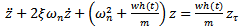 | (1) |
The following compact notations are used in equation (1);  and
and  . With the substitutions
 made, equation (1) could be put in state differential equation form as
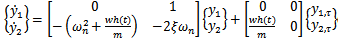 | (2) |
Where  . The details of generation of equations (1) and (2) are seen in literature[2, 3]
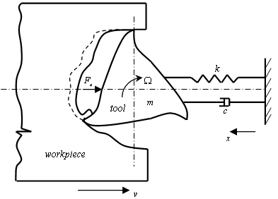 | Figure 1. Dynamical model of milling |
The quantity  is called the specific force variation for the system which is
  periodic where
  . The symbol
  is the spindle speed and
  is the number of teeth of the end miller. Milling is thus a delayed Mathieu system. Specific force variation was derived for a slotting three tooth end miller (figure 1) to have the form[4]
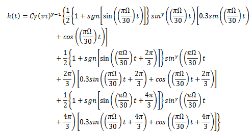 | (3) |
In equation (3)  is workpiece material cutting coefficient,
  is the cutting force feed exponent,
  is the prescribed feed speed and
  is cutting duration from initial feed. For the reference system having the parameters; cutting coefficient
 , feed speed
 , and spindle speed
  , the graphical portrayal of equation (3) becomes.
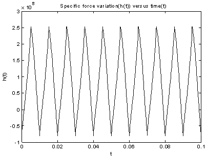 | Figure 2. specific force variation |
3. Time Finite Element Analysis
Stability of regenerative vibration using time finite elements involves dividing the period of cut into  time elements and estimating the perturbation motion of the system in each time element as a linear combination of trial functions. Within the present period of cut, the regenerative motion in the
  element becomes
  | (4) |
While for the delayed period of cut the motion was | (5) |
More works on time finite element analysis are found in literature[5, 6]. The trial functions utilized here are the polynomials 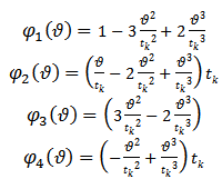 | (6) |
Where  is the local time of the
  time element of length
  . If uniform discretization is carried out then
  . A reader familiar with finite element analysis in space will notice that the hermit polynomials of equation (6) have the same form as a shape functions of a beam element of length
  (figure3) subjected to bending moment distribution
  when linear displacement
  is assumed to be a cubic polynomial function of local coordinates
  . Details exist in literature[7, 8, 9] that for such a beam element
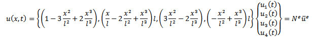 Where the elements of the row shape function matrix
  is seen to have the form of the trial functions of equation (6)
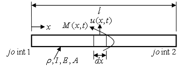 | Figure 3. A beam element |
Adopting uniform discretization, substitution of equations (4), (5) and (6) into equation (1) gives an error equation for the  element as
 | (7) |
Where  is the error of approximation arising from the use of trial functions and discretization process. Following the method of weighted residual, the integral of the weighted error over the
  element is set equal to zero giving
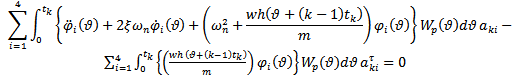 | (8) |
The weight functions  utilized are adopted from[5] to be
 | (9) |
Customarily nodal quantities are sought for in finite element method thus the nodal perturbations and their derivatives for the  element is seen from equations (4) and 96) to be
 | (10) |
The boundary condition that results from continuity between two adjacent time elements are | (11) |
For a slotting three tooth end miller under full immersion condition there is simultaneous engagement of adjacent teeth resulting in the extra boundary condition | (12) |
Substituting the weight functions  independently into equation (8) enables the formation of a local matrix equation for each element which in light of the boundary conditions (11) and (12) are assembled into the global matrix equation of form
 | (13) |
Where both  and
and  are seen to be
  matrices. As long as
  is non-singular, the global matrix equation can be put in the form
 | (14) |
For example, if three elements are to be used, the global matrix equation becomes 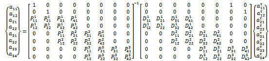 Where for the
  time element
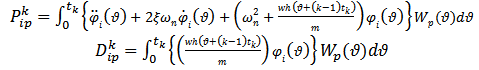 | (15) |
Equation (14) is a  -dimensional discrete time map of the system. It is seen that the nodal state vectors combine to form the global state vector of the discrete map. The matrix
  acts as a linear operator that transforms the delayed state
  to the present state
  . The matrix
  is called the monodromy matrix of the system. The nature of its eigenvalues also called characteristic multipliers determines the condition of stability of the system. The necessary and sufficient condition for asymptotic stability of the system is that each of the eigenvalues of the monodromy matrix has a magnitude that is less than one. In other words, all the eigen-values of the matrix
  must exist within a unit circle centred on at the origin of the complex plane. Since the magnitude of the eigen-values depends on the cutting parameter combination, the parameter space of the system has to be demarcated into stable and unstable domains. This is achieved on the cutting parameter plane of spindle speed and depth of cut by tracking the critical curve along which at least one of the characteristic multipliers lie on the unit circle. The two types of loss of stability (bifurcation) that are analytically and experimentally established for milling are[2, 3].1) Period two or period doubling or flip bifurcation in which the exit of the unit circle of the critical characteristic multiplier
  is at
is at  . 2) Secondary Hopf or Neimark-Sacker bifurcation which involves a pair of complex conjugate characteristic multiplier leaving the unit circle.
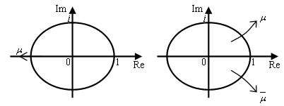 | Figure 4. a. Flip bifurcation; b. Secondary Hopf bifurcation |
4. Results and Discussions
Use is made of the monodromy matrix  of equation (14) to produce stability charts as shown in figure5 for the system under study with parameters
 .The region below the boundary curve is for stable chatter while that above it is for unstable chatter. For purposes of validation, each of the stability charts is overlaid with stability result of MATLAB dde23 of equation (1) for the studied system. Sample dde23 stable operating points are shown marked with star while the unstable points are marked with diamond. Each of the stability charts is given on the spindle speed(
 )-depth of cut (
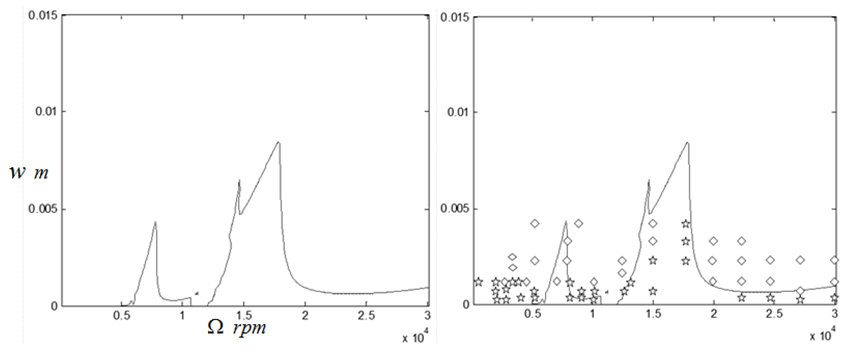
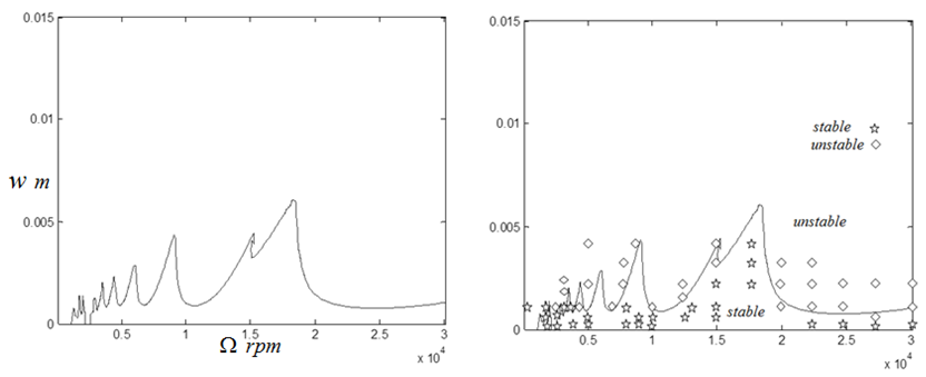
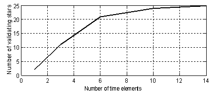
 ) parameter space. Use made of single time element results in a very inaccurate chart as seen in figure5a. There is a marked improvement in chart accuracy (though not reliable enough for practical application) when the number of time elements is increased to three as shown in figure 5b. System’s stability chart becomes further more accurate as the number of time finite element in analysis is increased to six. At this point the chart could be considered reliable enough for practical application as shown in figure 5c. Figure 5d shows that accuracy of stability chart continues to improve as the number of elements continues to increase. It is seen that figure 5d generated using ten elements is not only better define than figure 5c generated using six elements but also more accurate at low spindle speeds below 3000 rpm. The stability chart of figure 5e is generated using 14 elements. It is seen to have almost equal accuracy with that generated using ten time elements. For quantitative illustration the number of stable MATLAB dde23 solution (stars) that fall under each of the stability charts of figure6 is plotted on a line graph against the number of time elements used in analysis as shown in figure 6. It is seen for the studied full-immersion three tooth end-miller that above ten finite time elements only marginal gain in accuracy could be achieved by increase in number of elements.Back to Mr Berry’s problem that was mentioned at the introduction, it is seen clearly that charts of figures 5c, 5d and 5e reflect Mr Berry’s practical observation that there exist magic spindle speeds in the high speed range that cause an unstable chatter to quiet down. Optimal or highest depths of cut permissible for chatter free operation are achieved at the magic spindle speeds. If the studied system is a high speed system capable of spindle speed up to 20000rpm, the optimal productivity would occur at a spindle speed of 18000rpm at which a depth of about 5.5mm could comfortably be cut. It is seen from figure7 that there always exists a most productive depth of cut no matter what the spindle speed range of the machine is. What is needed for any tool-workpiece combination is experimental determination of the tool modal parameters; natural frequency
  and damping ratio
  and workpiece material parameter; cutting coefficient
  . With these parameters known, stability chart could be generated for the system by following the procedure outlined in this paper. With such a stability chart a machinist or operator of a milling machine would not encounter an impasse similar to that encountered by Mr Berry. Such equipped machinist will proactively control chatter by choosing from the chart a stable cutting parameter combination.
 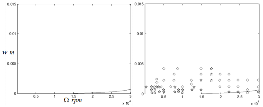 | Figure 5a. Stability chart of the syetem using one time finite element |
 | Figure 5b. Stability chart of the syetem using three time finite elements |
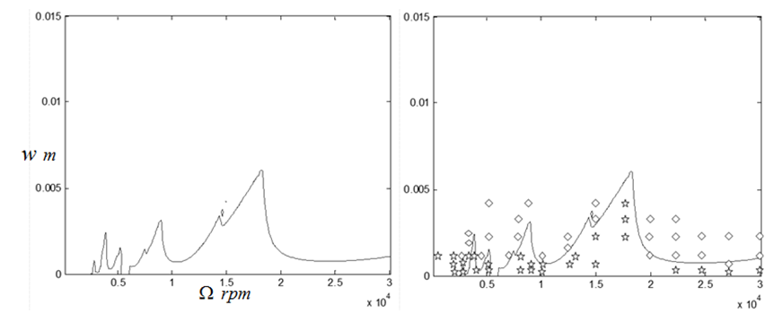 | Figure 5c. Stability chart of the syetem using six time finite elements |
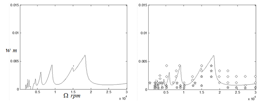 | Figure 5d. Stability chart of the syetem using ten time finite elements |
 | Figure 5e. Stability chart of the syetem using fourteen time finite elements |
 | Figure 6. Number of correctly placed stars against number of time finite elements |
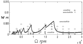 | Figure 7. Working stability chart of the system generated using fourteen time finite elements |
5. Conclusions
Stability chart of a slotting three tooth end miller was obtained using the method of time finite element analysis and compared with the result of MATLAB dde23 solution of milling equation. It was seen that close agreement exists between the two approaches when the number of time elements is high enough thus validating the resulting working chart that was generated using fourteen time elements. It is seen from the chart that that there exist magic spindle speeds that allow more productive dept of cuts. The magic spindle speeds allow optimal axial depths of cut. This result is seen to conform to milling stability characteristics observed by people working in workshop thus pointing to the validity of approach presented here for stability characterization a real tool-workpiece milling process. A machinist equipped with such a working stability chart will proactively control chatter while machining productively by choosing from the chart a stable cutting parameter combination. This type of stability analysis that leads to working stability chart precludes time loss that could have been occasioned by experimental trial and error method of determining productive spindle speeds.
References
| [1] | P. Zelinski, Chatter Control for the Rest of Us: Reprinted from Modern Machine Shop Magazine, Gardner Publications, Inc., 6915 Valley Ave., Cincinnati, Ohio 45244-3029, (2005). |
| [2] | T. Insperger, Stability Analysis of Periodic Delay-Differential Equations Modelling Machine Tool Chatter: PhD dissertation, Budapest University of Technology and Economics (2002). |
| [3] | C. G. Ozoegwu, Chatter of Plastic Milling CNC Machine: Master of Engineering thesis, Nnamdi Azikiwe University Awka (2011). |
| [4] | C. G. Ozoegwu, S. N Omenyi, C. C. Achebe and J. L. Chukwuneke, Chatter Stability Characterization of a Plastic end Milling CNC Machine, Accepted for publication in International Institute for Science, Technology and Education, (2011). |
| [5] | T. Insperger, B.P. Mann, G. Stepan, P.V. Bayly, Stability of up-milling and down-milling, part 1: alternative analytical methods, International Journal of Machine Tools & Manufacture 43 (2003), pp.25–34. |
| [6] | E. Butcher and B. Mann, Stability Analysis and Control of Linear Periodic Delayed Systems using Chebyshev and Temporal Finite Element Methods,http://mae.nmsu.edu/faculty/eab/bookchapter_final.pdf |
| [7] | R. J. Ashley, Finite Elements in Solids and Structures: An Introduction, Chapman and Hall London, 1992. |
| [8] | S. S. Rao, Mechanical Vibrations(4th ed.),Dorling Kindersley, India, 2004. |
| [9] | C. C. Ihueze, P. C. Onyechi, H. Aginam and C. G. Ozoegwu, Finite Design against Buckling of Structures under Continuous Harmonic Excitation, International Journal of Applied Engineering Research, ISSN 0973-4562 V, 6(12) (2011), pp. 1445-1460. |
 Abstract
 Reference
 Full-Text PDF
 Full-text HTML