P. Padmaja1, P. Pramod Chakravarthy2, Y. N. Reddy3
1Department of Mathematics, Prasad V Potluri Siddhartha Institute of Technology, Vijayawada, 520007, Andhra Pradesh, India
2Department of Mathematics, Visvesvaraya National Institute of Technology, Nagpur, 440010, India
3Department of Mathematics, National Institute of Technology, Warangal, 506004, India
Correspondence to: P. Pramod Chakravarthy, Department of Mathematics, Visvesvaraya National Institute of Technology, Nagpur, 440010, India.
| Email: |  |
Copyright © 2012 Scientific & Academic Publishing. All Rights Reserved.
Abstract
We consider a class of nonlinear singular perturbation problems of the form  with a boundary layer at one end point. Using the theory of singular perturbations, the original problem is reduced to an asymptotically equivalent first order initial value problem. Then, a variable step size initial value algorithm is applied to solve this initial value problem in a narrow region containing the layer region. The algorithm is based on the exact integration of a locally linearized problem (on a special non uniform mesh) exhibiting uniform convergence in for any x. Some problems are solved to demonstrate the applicability and efficiency of the algorithm. It is observed that the present method approximates the exact solution very well.
Keywords:
Singular Perturbation Problems, Boundary Layer, Variable Step Size, Locally Exact Integration
Cite this paper:
P. Padmaja, P. Pramod Chakravarthy, Y. N. Reddy, "A Numerical Scheme for Nonlinear Singularly Perturbed Two point Boundary Value Problems using Locally Exact Integration", American Journal of Computational and Applied Mathematics, Vol. 2 No. 6, 2012, pp. 306-310. doi: 10.5923/j.ajcam.20120206.09.
1. Introduction
Singular perturbation problems occur very frequently in fluid mechanics and other branches of applied Mathematics. The solution of the singularly perturbed boundary value problems has a multi scale character. The solution varies rapidly in some parts and varies slowly in some other parts. The numerical treatment of singular perturbation problems is far from trivial, because of the boundary layer behaviour of the solution. There are many physical situations in which the sharp changes occur inside the domain of interest, and the narrow regions across which these changes take place are usually referred as shock layers in fluid and solid mechanics, transition points in quantum mechanics, Strokes lines and surfaces in Mathematics. These rapid changes can not be handled by slow scales, but they can be handled by fast or magnified or stretched scales. A common strategy for dealing with this type of problems consists of dividing the domain of integration into two sub domains and then to apply a different scheme on each sub domain[1, 2]. In recent years a large number of analytical methods have been proposed[cf. Bender and Orszag[3], Kevorkian and Cole[4], O’ Malley[5], Nayfeh[6], Smith[7], Hu et.al[8]. Numerical methods based on initial value techniques and boundary value techniques are given in[9, 10, 11, 2]. Non linear single step methods for initial value problems were discussed by Van Niekerk[12]. A non standard explicit method for initial value problems is proposed by Ramos[13]. The more efficient, simpler computational techniques are required to solve singular perturbation problems. In general, finding a numerical solution of boundary value problems is more difficult than finding numerical solution of the corresponding initial value problems. Therefore it is better to convert the second order boundary value problem into asymptotically equivalent initial value problem. This replacement is significant from the computational point of view. A variable step size initial value algorithm is applied to solve this initial value problem in a narrow region containing the layer region. The algorithm is based on the exact integration of a locally linearized problem (on a special non uniform mesh) exhibiting uniform convergence in for any x.
2. Description of the Method
To describe the method, we consider a nonlinear singularly perturbed two-point boundary value problem of the form:  | (1) |
 | (2) |
where ε is a small positive parameter (0<ε<<1) and α, β are known constants. We assume that  are sufficiently continuously differentiable functions in
  Further more, we assume that (1)-(2) has a solution which displays a boundary layer of width O(ε) at
  for small values of ε.First we obtain the reduced problem by setting
  in equation (1) and solve it for the solution with an appropriate boundary condition. Let
  be the solution of the reduced problem
 We now set up the approximation equation to given equation (1) as follows
 | (3) |
where we simply replaced  by
by  in the last term of left hand side of the equation (1). Now we rewrite the equation (3) in the form
 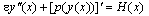 | (4) |
where 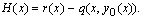 By integrating (4), we obtain
  | (5) |
where  and K is a constant to be determined.In order to determine K, we introduce the condition that the reduced equation of (5) should satisfy the boundary condition
  .
. | (6) |
Remark: This choice of K ensures that the solution of the reduced equation of (1)-(2) satisfies the reduced equation of (5). Hence, the equation (5) is a first order equation which is asymptotically equivalent to equation (1).We rewrite the equation (5) as | (7) |
 | (8) |
It is well known that the solution of (7) has singularity of boundary-layer type for definite conditions on the function  . On the other hand, classical integration schemes are usually ineffective in numerically solving (7) (see[14] for more details). However, there exist special schemes which present uniform convergence (in) for particular cases (see for the linear case[14], and[15,16] for Riccati-type), but these methods are also inadequate in general for nonlinear problems. Thus, to integrate problem (7) one must choose not only a difference scheme with good properties of stability ([14] A0 –stability, for example), but also a special non uniform mesh (on the interval[a, b]) which will depend on in the boundary layer zone and will be independent in the remainder. Algorithms of this type can be found in[17]. The one we shall give here also possesses these features.In order to know the behaviour of the solution of the singular perturbation problems in the boundary layer region, it is always suggestive to divide the original problem into two problems namely the inner region problem and the outer region problem and solve them separately. The general idea of domain decomposition process was originally introduced by Prandtl, which was later named as the method of matched asymptotic expansions. For many singular perturbation problems, a reduced problem is well defined and solution is known a priori. We divide the original problem into two problems, an inner region problem and an outer region problem. The inner region problem is defined over a narrow region
  and the outer region problem is defined over the interval
  Solution of the Inner Region ProblemThe inner region problem is given by (7)
  Mesh Selection StrategyWe form the non uniform grid in such a way that one wants to get more information about the solution of the boundary value problem (1) in the boundary layer region. This is quite natural because one would like to portray the behaviour of the solution in side the boundary layer region. The required step size can be determined directly according to the variation of the solution with in a time step as follows:If we stand at a point
  and we want to determine a point
  , which verifies
  , where δ is a user’s specified (constant) factor, then
  . The Numerical AlgorithmThe central idea of our algorithm is to integrate a linear problem obtained from (7) when
  is locally approximated by
  (with
(with  constants) on an interval whose length is chosen according to an estimation of
  ,where
  is a fixed parameter. In order to describe the first stage, we rewrite problem (7) in the following way:
  | (9) |
where  and
and  for some
  . Now if we integrate the linear part in (9) and impose that
  we obtain the function u given by
  where
where This function will approximate the exact solution of (7),
  , on the interval
  . For any x in
  we consider the approximate solution
  where
where Solution of the Outer Region ProblemThe solution of the reduced problem is considered as Outer solution.
3. Numerical Examples
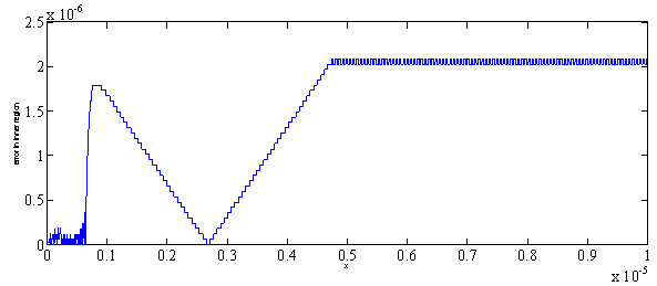
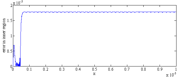
To demonstrate the applicability of the method, we have applied it to two nonlinear singular perturbation problems with left-end boundary layer. These examples have been chosen because they have been widely discussed in literature and because accurate solutions are available for comparison.Example 1 : Consider the following singular perturbation problem from Bender and Orszag[1], page :463; equations: 9.7.1;  We have chosen to use Bender and Orszag’s uniformly valid approximation (ref.[1], page: 463; equation: 9.7.6) for comparison. y(x)=loge(2/(1+x))-(loge2)e-2x/εFor this example, we have boundary layer of thickness O(ε) at x=0.(cf. Bender and Orszag [1]). The Maximum absolute error for Example 1 over a narrow region[0, 100ε] when δ=0.01is presented in Table 1 for ε=10-3 , ε=10-4 , ε=10-5 , ε=10-6 and ε=10-7 respectively. Piecewise solution error is shown in fig.1, fig.2 for ε=10-5 and ε=10-7 respectively.Example 2: Now consider the following singular perturbation problem from Kevorkian and Cole[6], page:56; equations: 2.5.1;
  We have chosen to use the Kivorkian and Cole’s uniformly valid approximation (Kevorkian and Cole[6]; pages 57 and 58; equations: 2.5.5, 2.5.11 and 2.5.14) for comparison.y(x)=x+c1tanh(c1(x/ε +c2)/2) Where c1=2.9995 and c2=(1/c1)loge[(c1-1)/(c1+1)]For this example also we have a boundary layer of width O(ε)at x=0.(cf. Kevorkian and Cole[6]).The Maximum absolute error for Example 2 over a narrow region[0, 100ε] when δ=0.01is also presented in Table 1 for ε=10-3 , ε=10-4 , ε=10-5 , ε=10-6 and ε=10-7 respectively. Piecewise solution error is shown in fig.3, fig.4 for ε=10-5 and ε=10-7 respectively.
| Table 1. Maximum absolute error over a narrow region [0, 100ε] when δ=0.01 |
| | ε | 10-3 | 10-4 | 10-5 | 10-6 | 10-7 | | Example 1 | 4.982948E-04 | 5.155802E-05 | 6.258488E-06 | 2.086163E-06 | 2.086163E-06 | | Example 2 | 3.457069E-04 | 4.577637E-05 | 1.788139E-05 | 1.788139E-05 | 1.788139E-05 |
|
|
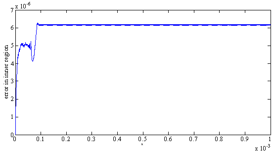 | Figure 1. Error plot for Example 1 for |
 | Figure 2. Error plot for Example 1 for 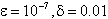 |
 | Figure 3. Error plot for Example 2 for  |
 | Figure 4. Error plot for Example 2 for  |
4. Discussion and Conclusions
In this article, we present a numerical method for solving a class of nonlinear singular perturbation problems using locally exact integration. Using the theory of singular perturbations, the original problem is reduced to an asymptotically equivalent first order initial value problem. This is significant from the computational point of view. In order to know the behaviour of the solution of the singular perturbation problems in the boundary layer region, it is always suggestive to divide the original problem into two problems namely the inner region problem and the outer region problem and solve them separately. A variable step size initial value algorithm is applied to solve this initial value problem in a narrow region containing the layer region. The algorithm is based on the exact integration of a locally linearized problem exhibiting uniform convergence in for any x. Piecewise solution error is shown in figures for different value of ε. The solution of the reduced problem is considered as Outer solution. This method is very easy to implement on any computer with minimum problem preparation. To support the applicability of the method we have implemented the present method on two non-linear examples with left-end boundary layer by taking different values of ε. Maximum absolute error in the inner region is presented in tables. It can be observed from the results that the present method agrees with exact solution very well, which shows the efficiency of the method.
References
| [1] | Natesan, S., Vigo-Aguiar, J., Ramanujam, N., A numerical algorithm for singular perturbation problems exhibiting weak boundary layers, Comput. Math. Appl. 45 (2003) 469 – 479. |
| [2] | Robert, S. M., A Boundary-Value Technique for Singular Perturbation Problems, Journal of Mathematical Analysis and Applications, Vol. 87(1982) 489-508. |
| [3] | Bender, C.M., and Orszag, S. A., Advanced Mathematical Methods for Scientists and Engineers, Mc. Graw-Hill, New York, 1978. |
| [4] | Kevorkian, J., and Cole, J. D., Perturbation Methods in Applied Mathematics, Springer-Verlag, New York, 1981. |
| [5] | O’ Malley, R. E., Introduction to Singular Perturbations, Academic Press, New York, 1974. |
| [6] | Nayfeh, A. H., Perturbation Methods, Wiley, New York, 1973. |
| [7] | Smith, D. R., Singular-Perturbation Theory an Introduction with Applications, Cambridge University Press, Cambridge, 1985. |
| [8] | Hu, X.C., Manteuffel, T.A., Mccormick, S., and Russell, T.F., Accurate discretization for singular perturbations: the one-dimensional case, SIAM Journal of Numerical Analysis, vol 32. No.1 (1995) 83-109. |
| [9] | Kadalbajoo, M. K., and Reddy, Y. N., Initial-Value Technique for a Class of Nonlinear Singular Perturbation Problems, Journal of Optimization Theory and Applications, Vol. 53 (1987) 395-406. |
| [10] | Kadalbajoo M.K. and Devendra Kumar: A non –linear single step explicit scheme for non-linear two point singularly perturbed boundary value problems via initial value technique, Applied Mathematics and Computation, Vol 202 (2008) 738-746. |
| [11] | Reddy, Y.N. and Pramod Chakravarthy, P., Method of Reduction of Order for Solving Singularly Perturbed Two-Point Boundary Value Problems, Applied Mathematics and Computation,Vol. 136 (2003) 27-45. |
| [12] | Van Niekerk, F.D., Non linear one step methods for initial value problems, Comput. Math. Appl. 13 (1987) 367-371. |
| [13] | Higinio Ramos, A non standard explicit integration scheme for initial value problems, Applied Mathematics and Computation, Vol. 189 (2007) 710 -718. |
| [14] | Doolan, E.P., Miller, J.J.H., Schilders, W.H.A., Uniform numerical methods for problems with initial and boundary layers, Boole press, Dublin, 1980. |
| [15] | Carroll, J., Exponentially fitted one step methods for the numerical solution of the scalar Riccati equation, J. Comput. Appl. Math. , 16(1) (1986) 9-25. |
| [16] | O’Reilly, M.J., A uniform scheme for the singularly perturbed Riccati equation, Numer. Math. 50 (4) (1987) 483-501. |
| [17] | Boglaev, I.P., Numerical integration of a singularly perturbed Cauchy problem for an ordinary differential equation, Zh. Vychisl. Mat. I Mat. Fiz. 25 (7) (1985) 1009-1022. |
 Abstract
 Reference
 Full-Text PDF
 Full-Text HTML