1. Introduction

The prey predator relationship still continues to be one of the main themes in mathematical ecology due to its complex dynamic behavior. Many prey predator models have been studied considering different types of functional responses [1,2,3]. It is seen that the invasion or introduction of exotic species in general disrupt the trophic dynamics of native interacting prey-predator species systems.

Introduced predators usually have a dramatic effect on native prey, usually the cause of native species extinction[4, 5, 6]. The harm caused by the introduced predators is broadly known and control programs are largely identified as the best way to restore ecosystems[7]. Many authors have studied effect of exotic predator on native prey species[8,9,10].

Dynamical consequences of predator interference in a tri-trophic model food chain is investigated by R K Naji et al[11]. Three-species food-chain model with Beddington DeAngelis type functional response has been studied by Wang and Zhao[12].

Meng Fan et al.[9] investigated the dynamical interaction among prey (bird), mesopredator (rat), and superpredator (cat) and developed a prey-mesopredator-superpredator (i.e. bird-rat-cat) BRC model, where the predator’s functional response is derived based on classical Holling’s time budget arguments. They have explored possible control strategies to save or restore the bird by controlling or eliminating the rat or the cat when the bird is endangered. They do not show under what conditions all the three species (BRC) will coexist and global stability analysis of interior equilibrium point is also not carried out.

In view of the above, the main purpose of this paper is to construct a general model to study the effect of exotic predator on a system consisting of a native prey population and a native predator population by considering Holling type two functional response with exotic predator interference for native predator population and Beddington type functional response for exotic predator population.

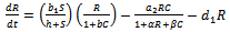
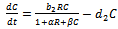
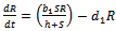
2. Basic Assumptions and Mathematical Model

Let denotes the density of native prey population, denotes the density of native predator population and denotes the density of exotic predator population. We assume that r and k are growth rate and carrying capacity of native prey population respectively. and are death rate of native predator population and exotic predator population respectively. b is the interference due to exotic predator population. is the predation rate of native prey population by native predator population. is the growth rate of native predator population due to predation of native prey population. is the predation rate of native predator population by exotic predator population. is the growth rate of exotic predator population due to predation of native predator population. h is the half saturation constant of native prey population. w is the wasting time to searching native predator by exotic predator. is the handling time to handle native predator by exotic predator. In view of above, the resultant system dynamics is governed by the following system of differential equations:

Model 1 (With exotic species)

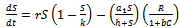(1)

(2)

(3)

With initial conditions and where and are positive constants.

In the absence of exotic predator species the above system (1) – (3) is governed by the following system of differential equations:

Model 2 ( Without exotic species)

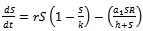(4)

(5)

With initial conditions and

3. Equillibria of the System

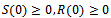
In this section, we analyze the system of equation (4) – (5) under the initial conditions. We find all the possible equillibria of the system of equation (4) – (5). The system has three feasible equillibria, namely

(i) Trivial equilibrium point

(ii) Axial equilibrium point

(iii) Positive interior equilibrium point

Where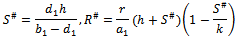

The positive equilibrium point exist if

We now analyze the system of equation (1) – (3) under the initial conditions. The system has four feasible equilibria, namely

(i)Trivial equilibrium point

(ii)Axial equilibrium point

(iii)Boundary equilibrium point

where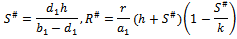

The boundary equilibrium point exist if

(iv)Positive interior equilibrium point

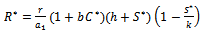
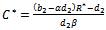
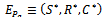where

(6)

(7)

(8)

The Positive interior equilibrium point exist if and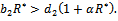

Now, we will study the existence of positive interior equilibrium point

Put value of from equation (7) in equation (6) we get,

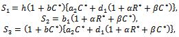
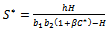(9)

where

Putting value of from equation (7) and putting value of from equation (9) in equation (8) we get

where

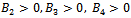Therefore unique positive root if and

4. Dynamic Behaviour of the System

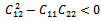
The following results may be noted regarding the local stability of the equilibria of the model 2 given by (4)-(5).

(1). Equilibrium point of the model is unstable in the absence of exotic species.

(2). Equilibrium point of the model is stable when there is no exotic species present in the system if

(3). Interior equilibrium point of the model is locally asymptotically stable when there is no exotic species present in the system if is satisfied.

The following results may be noted regarding the local stability of the equilibria of the model 1 given by (1)-(4).

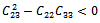
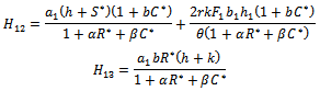
(1). Equilibrium point of the model is unstable in the presence of exotic species.

(2). Equilibrium point of the model is stable when exotic species is present in the system if

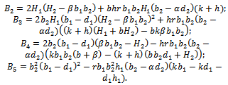
(3). Equilibrium point of the model is stable when exotic species is present in the system if and are satisfied.

(4). For the sake of simplicity, the equilibrium points of the system (1)-(3) is shifted to new points through transformations

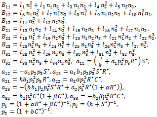
In term of the new variables, the dynamical system (1)-(3) can be written as in matrix form as

(10)

where dot cover denotes the derivative with respect to time. Here is the linear part of the system and represents the nonlinear part. Moreover,

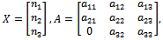(11)

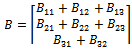(12)

where

The eigen values of the matrix help to understand the stability of the system. The characteristic equation for the variational matrix is given by

(13)

where

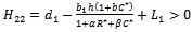
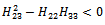
Using the Routh-Hurwitz criteria, we derive that the equilibrium point is locally asymptotically stable, if and are being satisfied.

Now, we are in a position to make an attempt to find out the condition under which the system undergoes Hopf-bifurcation[13]. For this purpose, we choose the parameter ‘’ as bifurcation parameter as it plays a crucial role to describe predation rate of native predator population by exotic predator population. We shall now apply the Liu’s criteria[14] to obtain the conditions for small amplitude periodic solution arising from Hopf-bifurcation. As the equilibrium population densities are function of ‘’, the coefficient of the characteristic equation (13) is a function of parameter ‘’ and hence we can use the notation for. Now noting that the quantities’s are smooth function of parameter, ‘ ’we first state for our case, the definition of a simple Hopf-bifurcation.

If a crucial value of parameter ‘’ is found such that (i) a simple pair of complex conjugate eigenvalues of characteristic equation (13) exist, say, such that they becomes purely imaginary at, i.e. 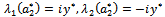with whereas the other eigen value remain real and negative; and the transversality condition (ii) is satisfied, then at , we have a simple Hopf-bifurcation. Without knowing eigen value[14] proved that (referring the result to the current case): if are smooth function of the parameter ‘’ in an open interval containing such that the following condition hold.

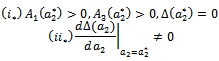Then and are equivalent to conditions and for the occurrence of a simple Hopf-bifurcation at Hence we can propose the following theorem:

Theorem 4.1 If a critical value of parameter ‘’ is found such that and further (where prime denotes differentiation with respect to) then system (1)-(3) undergoes Hopf-bifurcation around

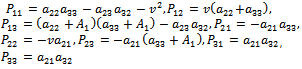
Next, we seek a transformation matrix which reduces the matrix to the form

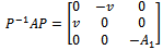(14)

Where the non-singular matrix is given as

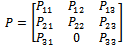(15)

where,

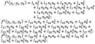
To achieve the normal form of (10), we make another change of variable, that is,

, where

Through some algebraic manipulation, (10) takes the form

(16)

where and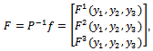

f is given by

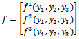(17)

where,

where,

Equation (16) is the normal form of (10) from which the stability coefficient can be computed. In (10), on the right hand side the first term is linear and second one is nonlinear in For evaluating the direction of bifurcating solution, we can evaluate the following quantities at and origin

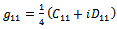(18)

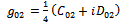(19)

(20)

(21)

(22)

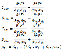
Thus, we can determine from (18),(19),(20), and (22), respectively. Thus, we can compute the following values:

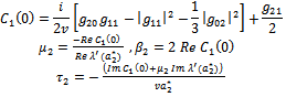(23)

which determine the qualities of bifurcation periodic solution in the center manifold at the critical value.

Theorem 4.2: The parameter determine the direction of the Hopf-bifurcation[15] if , then the Hopf-bifurcation is supercritical (subcritical) and the bifurcation periodic solutions exist for 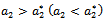; determine the stability of bifurcating periodic solution, the bifurcation periodic solutions are orbitally asymptotically stable (unstable) if; determine the period of the bifurcating periodic solution; the period increase (decrease) if.

5. Boundedness of the System

Lemma 5.1 All the solutions of system (4)-(5) with the positive initial condition are uniformly bounded within the region

where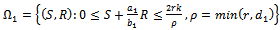

is a region of attraction.

Proof. Proof is obvious.

Lemma 5.2 All the solutions of system (1)-(3) with the positive initial condition are uniformly bounded within the region

where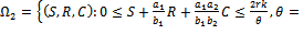

is a region of attraction.

Proof. We assume that the right hand sides of the system (1)-(3) are smooth function of 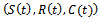of Let and be any solution with positive initial condition.

From equation (1), we obtain

then by usual comparison theorem[16]

We consider a time dependent function

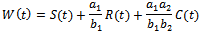The time derivative of along the solution of the system (1)-(3) is

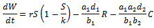Since, the above expression reduces to

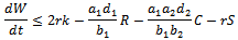Taking , we get

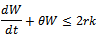Applying comparison theorem[17] we obtain

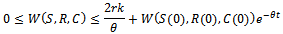and for,

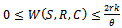
Therefore all the solutions of system (1)-(3) initiated at enter into the region

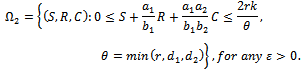Thus all the solutions of system (1)-(3) are uniformly bounded at

This completes the proof of the lemma.

6. Global Stability Analysis of the Interior Equilibrium Point

Theorem 6.1: The positive interior equilibrium point of the model 2 is globally asymptotically stable in absence of exotic predator species if is satisfied.

Proof: Proof is obvious.

Theorem 6.2: If the following inequalities hold

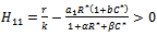(24)

(25)

(26)

where

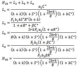
is globally asymptotically stable with respect to solutions initiating in the interior of the positive orthant. Proof: Consider the following positive definite function

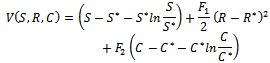where are positive constants to be chosen appropriately.

Differentiating with respect to t, we get

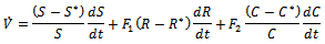Substituting values of and from the system of equations (1)-(3) in the above equation and after doing some algebraic manipulation, we get

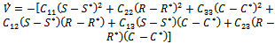where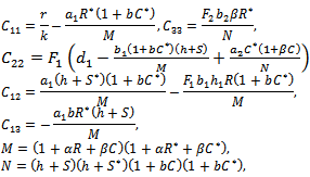

Then a sufficient conditions[18] for to be negative definite is that

(27)

(28)

(29)

(30)

(31)

hold.

Choosing and such a way

(32)

(33)

where

conditions (32) and (33) hold. However (32) implies (29) and (33) implies (30). Then above sufficient conditions reduce into the following inequalities.

(34)

(35)

(36)

However (24) implies (34), (25) implies (35) and (26) implies (36). Hence is negative definite and so is a Liapunov function with respect to, proving the theorem.

7. Simulation Analysis

We have gained analytical understanding of possible dynamics of the native prey-predator, exotic predator model. We now perform some simulation work for the model 2 with set of parameters.

For this choice of parameters we get a unique co-existing equilibrium point of Model 2 along with and hence is locally asymptotically stable (see Figure 1(a), 1(b)). We now perform simulation work for the model 1 with set of parameters.

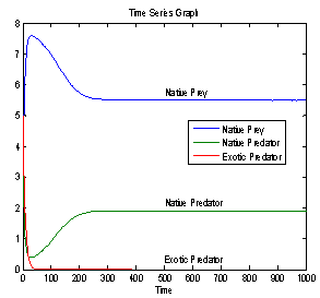
For this choice of parameters we get a unique co-existing equilibrium of Model 1 along with and hence is locally asymptotically stable (see Figure 4(a), 4(b)). Now, we discuss the dynamical behaviour of the model 1 by varying the parameter taking the above set of parametric values. For this, we find out the positive roots of the equation and we obtain three positive roots of this equation i.e. (See Figure 7(a), 7(b), 7(c)). At one pair of eigen values of the characteristic equation (13) are of the form, where is a positive real number and hence the system (1)-(3) undergoes a Hopf-bifurcation at. For we get. From these values, it follows from (23) that and showing that the bifurcation takes place when crosses to the right and the corresponding periodic orbits are orbitally asymptotically stable (See Figure 5(a) and 5(b) for). For we get From these values, it follows from (23) that and showing that the bifurcation takes when crosses to the left and the corresponding periodic orbits are orbitally asymptotically unstable. The system (1)-(3) undergoes a Hopf-bifurcation at. For we get From these values, it follow from (23) that and showing that the bifurcation takes when crosses to the right , and the corresponding periodic orbits are orbitally asymptotically stable (See Figure 6(a) and 6(b)

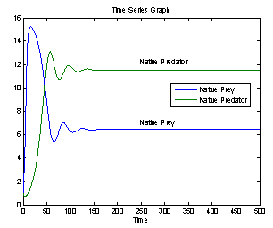Figure 1(a). Stable population distribution for native prey and native predator species

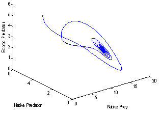
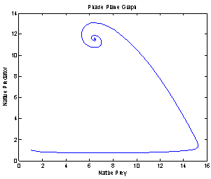Figure 1(b). Phase space graph between native prey and native predator species

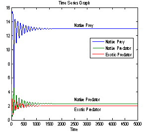
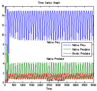
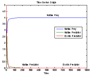Figure 2. Time series graph for native prey , native predator and exotic predator species

Figure 3. Time series graph for native prey , native predator and exotic predator species

Figure 4(a). Stable population distribution for native prey , native predator and exotic predator species

Figure 4(b). Phase space graph for native prey , native predator and exotic predator species

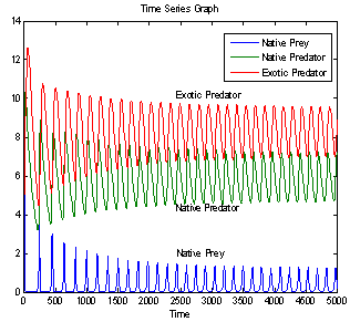Figure 5(a). Time series graph for native prey , native predator and exotic predator species at

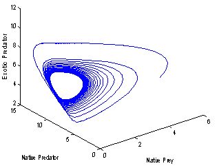Figure 5(b). Phase space graph for native prey , native predator and exotic predator species at

Figure 6(a). Time series graph for native prey , native predator and exotic predator species at

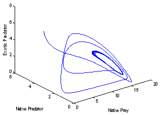Figure 6(b). Phase space graph for native prey , native predator and exotic predator species at

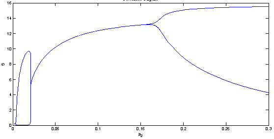Figure 8(a). Bifurcation diagram of the native prey species with respect to predation rate

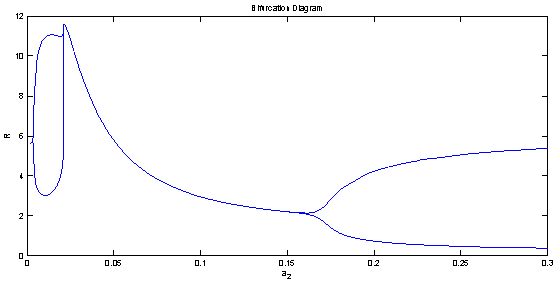Figure 8(b). Bifurcation diagram of the native predator species with respect to predation rate

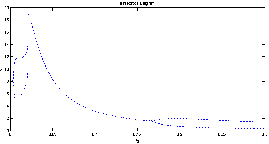Figure 8(c). Bifurcation diagram of the exotic predator species with respect to predation rate

8. Conclusions

In this paper, a mathematical model is proposed to study the effect of exotic predator population on a native prey-predator species system. The local stability analyses of all the feasible equilibria are carried out. We observed that if the axial equilibrium point of model 2 is stable then interior equilibrium point does not exist and if interior equilibrium point of model 2 exists then axial equilibrium point is unstable. From the stability of axial equilibrium point E_Ae [see figure 2], it may be concluded that native prey population will survive and native and exotic population may go to extinction. From the stability of boundary equilibrium point E_Be [see figure 3], it is observed that the exotic predator population will not survive and consequently native prey-predator population will coexist. The global stability analysis of both the models 1 and 2 are carried out, and the possibility of Hopf- bifurcation of the interior equilibrium point is investigated. We observed that the positive interior equilibrium point is stable for and (see figure 8(a), 8(b), 8(c)). The switching in stability behaviour based on predation rate of exotic predator; is also observed (see figure 8(a), 8(b), 8(c)). We also determine the stability and direction of periodic bifurcation from the positive equilibrium at the critical point. Finally we conclude that invasion of exotic predator is harmful to native prey-predator system. We also clear that exotic predator is harmful to native predator and helpful to native prey. The predation rate of exotic predator creates complex phenomena in the system. The present work may be extended by considering the migration of the population.