-
Paper Information
- Next Paper
- Previous Paper
- Paper Submission
-
Journal Information
- About This Journal
- Editorial Board
- Current Issue
- Archive
- Author Guidelines
- Contact Us
American Journal of Computational and Applied Mathematics
p-ISSN: 2165-8935 e-ISSN: 2165-8943
2012; 2(6): 276-289
doi: 10.5923/j.ajcam.20120206.06
Modelling Effect of Toxic Metal on the Individual Plant Growth: A Two Compartment Model
 Abstract
 Reference
 Full-Text PDF
 Full-Text HTML
O. P. Misra, Preety Kalra
School of Mathematics and Allied Sciences, Jiwaji University, Gwalior, 474011, M.P., India
Correspondence to: Preety Kalra, School of Mathematics and Allied Sciences, Jiwaji University, Gwalior, 474011, M.P., India.
| Email: |  |
Copyright © 2012 Scientific & Academic Publishing. All Rights Reserved.
A two compartment mathematical model for the individual plant growth under the stress of toxic metal is studied. In the model it is assumed that the uptake of toxic metal adsorbed on the surface of soil by the plant is through root compartment thereby decreasing the root dry weight and shoot dry weight due to decrease in nutrient concentration in each compartment. In order to visualize the effect of toxic metal on plant growth, we have studied two models that is, model for plant growth with no toxic effect and model for plant growth with toxic effect. From the analysis of the models the criteria for plant growth with and without toxic effects are derived. The numerical simulation is done using Matlab to support the analytical results.
Keywords: Nutrient Concentration, Dry weight, Toxic metal, Model, Equilibria, Stability
Cite this paper: O. P. Misra, Preety Kalra, "Modelling Effect of Toxic Metal on the Individual Plant Growth: A Two Compartment Model", American Journal of Computational and Applied Mathematics, Vol. 2 No. 6, 2012, pp. 276-289. doi: 10.5923/j.ajcam.20120206.06.
Article Outline
1. Introduction
- Soil normally contains a low concentration of heavy metals such as copper (Cu) and zinc (Zn), which are the essential macronutrients for the optimum growth of the plants. Metals such as cadmium (Cd), arsenic (Ar), chromium (Cr), lead (Pb), nickel(Ni), mercury(Hg) and selenium (Se) toxic to plants are not usually found in agricultural soil[1]. Over the last few years, the level of heavy metals are increasing in the agricultural fields as a consequence of increasing environmental pollution from industrial, agricultural, energy and municipal wastes. A reduction in plant growth has been observed due to the presence of elevated levels of heavy metals like cadmium, arsenic, nickel, lead and mercury[2]. Cadmium (Cd) is among the most widespread heavy metals found in the surface soil layer which inhibits the uptake of nutrients by plants and as well as its growth[3]. The inhibition of plant growth can be caused by the phytotoxic effect of cadmium on different processes in plants, including respiration, photosynthesis, carbohydrate metabolism and water relation[4]. Cadmium (Cd) ia a toxic metal, causing phytotoxicity, and its uptake and accumulation in plants causes reduction in photosynthesis, diminishes water and nutrient uptake[5]. Heavy metals interfere with the uptake and distribution of essential mineral nutrients in a plant, causing deficiencies and nutrient imbalance[6]. The toxic metals in the soil system could result in the leaching of essential cation away from the rooted zone, decreasing plant nutrient uptake causing root damage[7]. Cadmium inhibits root and shoot growth and yield production, affects nutrient uptake and homeostasis. Cadmium is a highly toxic, metallic soil contaminant, which adversely affects the plant growth especially at early stage reducing the crop production[8]. The reduction of dry weight by
 toxicity could be the direct consequence of the inhibition of chlorophyll synthesis and photosynthesis[9]. Excessive amount of
  may also cause decrease in uptake of nutrient elements, inhibition of various enzyme activities, induction of oxidative stress including alterations in the enzymes of the antioxidant defense system[10]. Aluminium (Al) interferes with the uptake, transport and utilization of essential nutrients including
  ,
,  ,
,  ,
,  ,
,  ,
,  ,
,  and
and  in plant system[11]. Metals inhibit the activities of several enzymes, seed germination and seedling growth[12-15]. Seed gemination inhibition by heavy metals has been reported by many researchers[16-18]. Agricultural research almost completely rely upon experimental and empirical works, combined with statistical analysis and very few mathematical modelling analysis has been carried out in this direction[3-4],[19-20]. Many of the models that are currently used by agronomists and foresters to predict harvests and schedule fertilization, irrigation and pesticides application are of empirical form. A major limitation in all these approaches is the unpredictability of the environmental inputs[21]. Thornley initiated the work related to the mathematical modelling of individual plant growth processes and mathematical models were applied to a wide variety of topics in plant physiology[22]. The majority of these focuses on processes that are modelled independently such as photosynthesis, fluid transport, respiration, transpiration and stomatal response and the general goal of the models was to predict the effect of a variety of environmental factors, including radiation input, humidity, wind, CO2 concentration and temperature on these process rates. The soil-nutrient-plant interaction represents a good example of a relationship that operates at individual, population, and ecosystem levels. Nutrients influence individual plant growth, which has subsequent effect on population growth dynamics which in turn influence production of standing crop. The models that have been developed to describe the growth of individual plants in crop has been classified by Benamin and Hardwick[23], according to the assumption that how resources are shared. A continuous-time model for the growth and reproduction of a perennial herb with discrete growing season is considered in[24] and optimal resource allocation in perennial plants has been determined and studied. In the paper[25], a transient three-dimensional model for soil water and solute transport with simultaneous root growth, root water and nutrient uptake is studied and discussed. In this paper, authors have presented a model to study the interactive relationships between changing soil-water and nutrient status and root activity. The authors in the paper[19] have studied the influence of acid deposition on forests by means of a mathematical model taking the state variables as forest dry weight, aluminium concentration in trees and soil, and proton concentration in soil. Referrence[3] have given a mathematical model to study the effect of cadmium (Cd) on nutrient uptake by crop such as Barley and have shown through their model that how the accumulation of Cd in plants inhibit its growth rate. Experimental and mathematical simulation to study the effects of toxic metal; cadmium on the plant growth promoting rhizobacteria and plant interaction have been carried out by[4]. Nitrogen dynamics in soil, its availability to the crop and the effects of nitrogen deficiency on crop performance were studied in the model given by the researchers[26]. A non-spatial, size- structured continuum model of plant growth, without focusing on a particular species, but with emphasis on a dense tree-dominated forest is considered and studied by[27] and in this paper a closed form solution for the equilibrium size density distribution is obtained along with the analytical conditions for communities persistence. Crops and vegetables grown on polluted soil accumulate heavy metals that cause decrease in their yield, and in order to study the uptake of heavy metals and its accumulation by crops, mathematical models can be used. In paper[20], a study has been conducted through mathematical model to understand the cadmium uptake by radish, carrot, spinach and cabbage. In this paper a dynamic macroscopic numerical model for heavy metal transport and its uptake by vegetables in the root zone is considered and analysed numerically. A very few mathematical models to study the effects of toxic metal on plant growth exist[3-4],[19-20].In view of the above, therefore in this paper, a two compartment mathematical model for the plant growth under the stress of toxic metal is proposed and analyzed. For the modelling purpose, the plant is divided into root and shoot compartments in which the state variables considered are nutrient concentration and dry weight. In the model it is assumed that the uptake of toxic metal adsorbed on the surface of soil by the plant is through root compartment thereby decreasing the root dry weight and shoot dry weight due to decrease in nutrient concentration in each compartment. In the model it is further assumed that the maximum root dry weight and shoot dry weight decrease due to the presence of toxic metal in root compartment. From the analytical and numerical analysis of the model the criteria for plant growth under the stress of toxic metal are derived.
 2. Mathematical Model
- Model 1 (Model with no toxic effect):In this model the plant growth dynamics is studied by assuming that the plant is divided into root and shoot (stem, leaf, flower) compartments in which the state variables associated with the each compartment are nutrient concentration and dry weight. Let
 and
and  denote the root dry weight and shoot dry weight respectively.
  and
and  denote the nutrient concentration in root and shoot respectively. With these notations, the mathematical model of the plant growth dynamics is given by the following system of nonlinear differential equations:
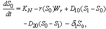 | (1) |
 | (2) |
 | (3) |
 | (4) |
 | (5) |
 In the present analysis we assume the following forms for growth functions
  and
and  [22],[28] :
  | (6) |
 is the utilization coefficient.
  and
and  are the proportion of total dry weight allocated to root and shoot dry weight respectively.
  and
and  are the resource-saturated rates of resource uptake per unit of root and shoot dry weight respectively.
  and
and  are half saturation constants.
  is the rate of supply of nutrient.
  is the specific gross photosynthetic rate[22].
  is the fraction of shoot in the form of leaf tissue.
  is senescence constant.
  is the maximum age of shoot of plant.
  is the specific leaf area of whole plant.
  is the light flux density incident on the leaves in shoot compartment.
  is the
  density in plant.
  is the rate of senescence of the photosynthesis. β is the photochemical efficency. γ is the conductance to
  .
. and
and  represent the use of nutrient by root and shoot respectively[26]. In plant growth, it is considered that during the initial stage, i.e., during the lag phase, the rate of plant growth is slow. Rate of growth then increases rapidly during the exponential phase. After some time the growth rate slowly decreases due to limitation of nutrient. This phase constitutes the stationary phase . The terms
  and
and  are taken to account for the diminishing growth phase and stationary phase in the plant growth dynamics. Where,
  is the maximum root dry weight.
  is the maximum shoot dry weight.
  and
and  are nutrient limiting coefficients.
  and
and  represent the flux of nutrient from shoot to root and root to shoot respectively. Where,
  and
and  are transfer rates.
  represents the loss of nutreint due to leaching.
  represent the loss of nutrient due shedding of leaves.
  is leaching rate and
  is natural decay rate of
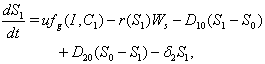
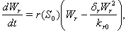
  .Model 2 (Model with toxic effect):In this model, the effect of toxic metal on plant growth dynamics is considered. Here, we assume that the nutrient concentration and dry weight are adversely effected by toxic heavy metal. Let
  is the concentration of toxic metal in soil and
  is the concentration of toxic metal adsorbed on the surface of soil. After incorporating the stress of toxic metal in the model 1 with the assumptions mentioned earlier in section 1, we get the following model 2:
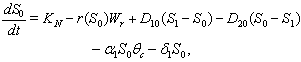 | (7) |
 | (8) |
 | (9) |
 | (10) |
 | (11) |
 | (12) |
 Here, we assume the following forms for
  ,
,  and uptake function
  [25]:
[25]: | (13) |
 ,
,  ,
,  ,
,  ,
,  ,
,  ,
,  ,
,  ,
,  ,
,  ,
,  ,
,  ,
,  and
and  , which are described as follows:
  is the input rate of heavy metals.
  is the first order rate constant.
  is the soil bulk density.
  is the linear adsorption and absorption coefficient.
  and
and  are decreasing rates of
  and
and  respectively due to
  .
. is the maximum uptake rate of
  .
.  is the Michaelis-Menten constant.
  is the first order rate coefficient.
  is the natural decay rate of
  due to soil depletion on account of natural process.
  is natural decay rate of
  . Here, all the parameters
  ,
,  ,
, 

 and
and  are taken to be positive constants.
3. Boundedness and Dynamical Behaviour
3.1. Analysis of Model 1
- Now, we show that the solutions of the model given by (1) to (4) are bounded in a positive orthant in
 . The boundedness of solutions is given by the following lemma.Lemma 3.1: All the solutions of model will lie in the region
  as
as , for all positive initial values
  ,where
  .Proof: By adding Eqs. (1) and (2), we get,
  where,
  and then by the usual comparison theorem we get as
 From Eq. (3), we get,
 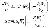 if
if  and then by the usual comparison theorem we get as
 Similarly from Eq. (4), we get,
  This complete the proof of lemma.Now we show the existence of the interior equilibrium
  of Model 1. The system of equations (1) - (4) has one feasible equilibria
  . The equilibrium
  of the system is obtained by solving the following equations,
 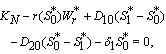 | (14) |
 | (15) |
 | (16) |
 | (17) |
 , where,
  | (18) |
 | (19) |
 and
and  can be obtained by solving the following pair of equations:
 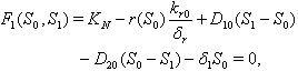 | (20) |
 | (21) |
 implies
 ,2.
,2.  implies
  3.
3.  implies
 4.
4.  implies
 where,
  and
and  .The two Eqs. (20) and (21) intersect each other in the positive phase plane satisfying
  for Eq. (20) and
  for Eq. (21), showing the existence of the unique interior equilibrium
  .From Eq. (15) as
  :
:  | (22) |
 of the model given by (1)-(4) and for this local and global stability analysis have been carried out subsequently.The characteristic equation associated with the variational matrix about equilibrium
  is given by
  | (23) |
 From the nature of the roots of the characteristic equation (23) we derive that the equilibrium point
  is always locally asymptotically stable.Now, we discuss the global stability of the interior equilibrium point
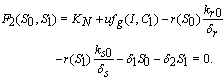
  of the system (1)-(4). The non-linear stability of the interior positive equilibrium is determined by the following theorem.Therorem 3.2: In addition to assumptions (6), let
  and
and  , satisfy in
 | (24) |
 and
and  less than 1. Then if the following inequalities hold
 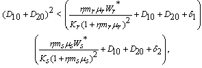 | (25) |
 | (26) |
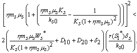 | (27) |
 is globally asymptotically stable with respect to solutions initiating in the interior of the positive orthant. Proof: Since
  is an attracting region, and does not contain any invariant sets on the part of its boundary which intersect in the interior of
  , we restrict our attention to the interior of
  . We consider a positive definite function about
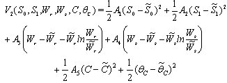

 Then the derivatives along solutions,
  is given by
 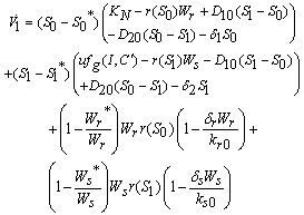 After some algebraic manipulations, this can be written as
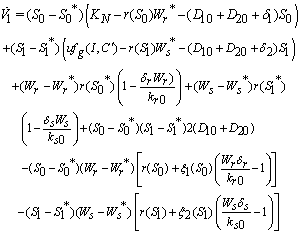 Where,
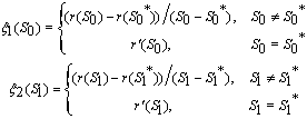 We note from (24) and the mean value theorem, that
 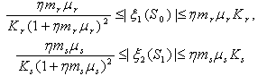 We know that
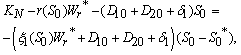
 Hence
Hence  can be written as the sum of three quadratic forms,
 Where,
 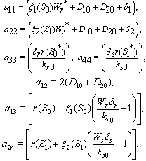 By Sylvester’s criteria we find that
  is negative definite if
 | (28) |
 | (29) |
 | (30) |
 is negative definite and so
  is a Liapunov function with respect to
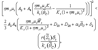
  , whose domain contains
  , proving the theorem.The above theorem shows, that provided inequalities (25) to (27) hold, the system settles down to a steady state solution.
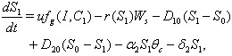
3.2. Analysis of Model 2
- Now, in the following we show that the solutions of model given by (7) to (12) are bounded in a positive orthant in
 . The boundedness of solutions is given by the following lemma.Lemma 3.3: All the solutions of model will lie in the region
  as
as  , for all positive initial values
  , where
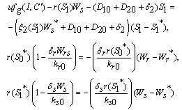
 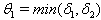 . Proof: By adding Eqs. (7) and (8), we get,
 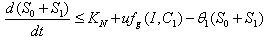 where,
 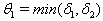 and then by the usual comparison theorem we get as
 From Eq. (9), we get,
 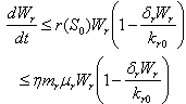 if
if  and then by the usual comparison theorem we get as
 Similarly from Eq. (10), we get,
  From Eq. (11), we get,
  Then by the usual comparison theorem we get as
 From Eq. (12), we get,
  Then by the usual comparison theorem we get as
 This complete the proof of lemma.Now, we find the interior equilibrium
  of Model 2. The system of equations (7) - (12) has one feasible equilibria
  . The equilibrium
  of the system is obtained by solving the following equations,
 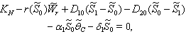 | (31) |
 | (32) |
 | (33) |
 | (34) |
 | (35) |
 | (36) |
 , where,
  | (37) |
 | (38) |
 | (39) |
 increases.The
  is given by the positive root of the equation
 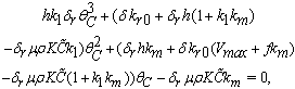 | (40) |
 and
and  can be obtained by solving the following pair of equations:
 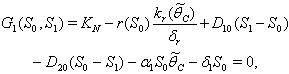 | (41) |
 | (42) |
 implies
 2.
2.  implies
  3.
3.  implies
 4.
4.  implies
 where,
  and
and  .The two Eqs. (41) and (42) intersect each other in the positive phase plane satisfying
  for Eq. (41) and
  for Eq. (42), showing the existence of the unique interior equilibrium
  .From Eq. (32) as
  :
:  | (43) |
 of the model given by (7)-(12) and for this local and global stability analysis have been carried out subsequently.The characteristic equation associated with the variational matrix about equilibrium
  is given by
 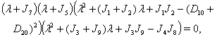 | (44) |


 From the nature of the roots of the characteristic equation (44) we derive that the equilibrium point
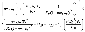
  is locally stable if
 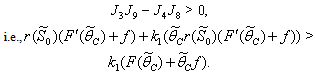 | (45) |
 of the system (7)-(12). The non-linear stability of the interior positive equilibrium state is determined by the following theorem.Therorem 3.4: In addition to assumptions (6) and (13), let
  ,
,  ,
,  ,
,  and
and  satisfy in
 | (46) |
 and
and  less than 1. Then if the following inequalities hold
 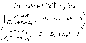 | (47) |
 | (48) |
 | (49) |
 | (50) |
 is globally asymptotically stable with respect to solutions intiating in the interior of the positive orthant. Proof: Since
 is an atttracting region, and does not contain any invariant sets on the part of its boundary which intersect in the interior of
  , we restrict our attention to the interior of
  .We consider a positive definite function about
 where,
  are arbitrary positive constants. Then the derivatives along solutions, is given by After some algebraic manipulations, this can be written as
 Where
Where We note from (46) and the mean value theorem, that
  and
and 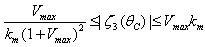 .We know that
 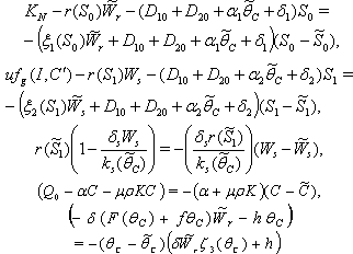 Hence
Hence  can be written as the sum of three quadratic forms
 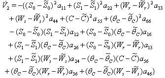 where
where 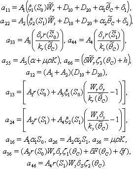 By Sylvester’s criteria we find that
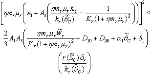
  is negative definite if
  | (51) |
 ,
,  ,
,  and
and  are satisfied due to arbitrary choice of
  ,
,  ,
,  and
and  respectively, and above conditions reduces to the following conditions:
  | (52) |
 | (53) |
 | (54) |
 | (55) |
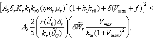
 is negative definite and so
  is a Liapunov function with respect to
  , whose domain contains
  , proving the theorem.The above theorem shows, that provided inequalities (47) to (50) hold, the system settles down to a steady state solution.
4. Numerical Example
- For the model 1, consider the following values of parameters-
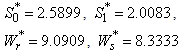
 For the above set of parametric values, we obtain the following values of interior equilibrium point
  -
- which is asymptotically stable (see Figure 1).Further, to illustrate the global stability of interior equilibrium
  of model 1 graphically, numerical simulation is performed for different initial conditions (see Table 1 and 2) and results are shown in Figures 2 and 3 for
  phase plane and
  phase plane respectively. All the trajectories are starting from different initial conditions and reach to interior equilibrium
  .
.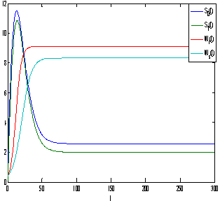 | Figure 1. Trajectories of the model 1 with respect to time (with no toxic effect) showing the stability behaviour |
|
 and
and  of model 1
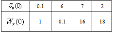
|
 and
and  of model 1
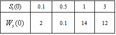
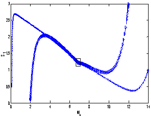
 | Figure 2. Phase plane graph for nutrient concentration in root S0 and root dry weight Wr at different initial conditions given in Table 1 for model 1 (with no toxic effect) showing the global stability behaviour |
 | Figure 3. Phase plane graph for nutrient concentration in shoot S1 and shoot dry weight Ws at different initial conditions given in Table 1 for model 1 (with no toxic effect) showing the global stability behaviour |
 we obtain the following values of interior equilibrium point
  as
as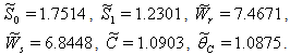 For the set of parametric values considered, the stability conditions given in Eq. (45) and Eqs. (47)-(50) are satisfied. Hence,
  is asymptotically stable (see Figure 4).
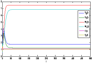 | Figure 4. Trajectories of the model 2 with respect to time (with toxic effect) showing the stability behaviour |
 of model 2 graphically, numerical simulation is performed for different initial conditions (see Table 3 and 4) and results are shown in Figures 5 and 6 for
  phase plane and
  phase plane respectively. All the trajectories are starting from different initial conditions and reach to interior equilibrium
|
|
 | Figure 5. Phase plane graph for nutrient concentration in root S0 and root dry weight Wr at different initial conditions given in Table 3 for model 2 (with toxic effect) showing the global stability behaviour |
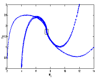 | Figure 6. Phase plane graph for nutrient concentration in shoot S1 and shoot dry weight Ws at different initial conditions given in Table 4 for model 2 (with toxic effect) showing the global stability behaviour |


5. Conclusions
- Equilibrium
 of model 1 is shown to be asymptotically stable (see Fig. 1). The equilibria
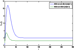
  of model 2 is shown to be asymptotically stable (see Fig. 4). From Figures 7(a) and 7(b), it may be noted that the equilibrium levels of nutrient concentrations in each compartment with no toxic effect are more than that of the equilibrium levels of nutrient concentrations in respective compartments when toxic effect is considered.
 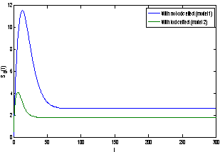 | Figure 7(a). Graph between nutrient concentration in root S0 and time t for model 1(with no toxic effect) and for model 2(with toxic effect) |
 | Figure 7(b). Graph between nutrient concentration in shoot S1 and time t for model 1(with no toxic effect) and for model 2(with toxic effect) |
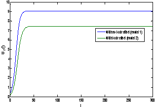 | Figure 8(a). Graph between root dry weight Wr and time t for model 1 (with no toxic effect) and for model 2(with toxic effect) |
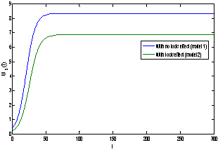 | Figure 8(b). Graph between shoot dry weight Ws and time t for model 1(with no toxic effect) and for model 2(with toxic effect) |
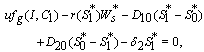
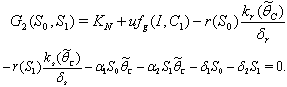
 and tolerance indices (Table 5), it is concluded that the root dry weight and shoot dry weight decrease as the input rate of toxic metal
  increases till
  is less than or equal to
  and upto this value the stability criteria is also preserved. Further, in case if
  increases from its threshold value
  then the stability condition given by Eq. (45) is voilated and equilibrium
  loses its stability. From the expressions (37) and (38) it may be noted that the root dry weight and shoot dry weight will decrease and may tend to zero with increasing
  . From Eqs. (22) and (43), it is concluded that for large
  , the nutrient concentration in shoot with toxic effect is less than that of nutrient concentration in shoot when no toxic effect is considered. The Figures 9(a) and 9(b) represent the dynamical behaviour of the of root dry weight and shoot dry weight with respect to
  . From these figures it is observed that the toxicity of the metal will adversely effect the plant growth in its early stages resulting in loss of crop productivity[8],[29].
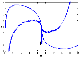
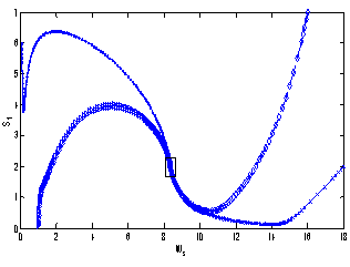
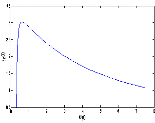 | Figure 9(a). Phase Plane Graph of root dry weight Wr and θC for model 2 |
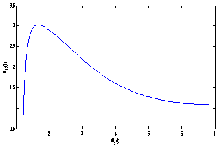 | Figure 9(b). Phase Plane Graph of shoot dry weight Wr and θC for model 2 |
References
| [1] | R. Tucker, D.H. Hardy, C.E. Stokes, Heavy Metals in North Carolina Soils, Occurance and Significance, N.C. Department of Agriculture and Consumer Services, Agronomics division, Raleigh, 2003. |
| [2] | R.H. Merry, K.G. Tiller, A.M. Alston, The Effects of Contamination of Soil with Copper, lead, Mercury and Arsenic on the Growth and Composition of Plants. Effects of Season, Genotype, Soil Temperature and Fertilizers, Plant Soil, Vol. 91, 115-128, 1986. |
| [3] | A. Brune, K. J. Dietz, A Comparative Analysis of Element Composition of Roots and Leaves of Barley Seedlings Grown in the Presence of Toxic Cadmium, Molybdenum, Nickel and zinc Concentration, J. Plant. Nutr, Vol. 18, 853-868, 1985. |
| [4] | V. N. Pishchik, N. I. Vorobyev, I. I. Chernyaeva, S. V. Timofeea, A. P. Kozhemyakov, Y. V. Alexeev, S. M. Lukin, Experimental and Mathematical Simulation of Plant Growth Promoting Rhizobacteria and Plant Interaction under Cadmium Stress, Plant and Soil, Vol. 243, 173-186, 2002. |
| [5] | L.S.D. Toppi, R. Gabbrielli, Response to Cadmium in hHgher Plants, Environ. Exp. Bot., Vol. 41, No. 2, 105-130, 1999. |
| [6] | S. Trivedi, L. Erdei, Effects of Cadmium and lead on the Aaccumulation of Ca2+and K+ and on the Influx and Ttranslocation of K+ Status, Physiol. Plant, Vol. 84, 94-100, 1992. |
| [7] | Misra, O. P., Sinha P., Rathore, S. K. S., 2008, Effect of Polluted Soil on the Growth Dynamics of Plant-Herbivour System: A Mathematical Model, Proc. Nat. Acad. Sci. India Sect, Vol. A 78, Pt.II. |
| [8] | S. Faizan, S. Kuusar, R. Perveen, Varietal Difference for Cadmium-induced Seedling Mortality, Foliar Toxicity Symptoms. Plant Growth, Proline and Nitrate Reductase Activity in Chickpea(Cicer Arietinum L), Biology and Medicine, Vol. 3, 196-206, 2011. |
| [9] | K. Padmaja, D.D.K. Prasad, A.R.K. Prasad, Inhibition of Chlorophyll synthesis in Phaseolus Vulgrais Seedlings by Cadmium Acetate Photosynthetica, Vol. 24, 399-405, 1990. |
| [10] | L.M. Sandalio, H.C. Dalurzo, M. Gomez, M. C. Romero-Puertas, L.A. Del Rio, Cadmium-induced Changes in the Growth and Oxidative Metabolism of Pea Plants. Journal of Experimental Botony, Vol. 52, 2115-2126, 2001. |
| [11] | R.T. Guo, G.P. Zhang, W.Y. Lu, H.P. Wu, , F.B. Wu, J.X. Chen, J.X. Zhou, Effect of Al on dry matter accumulation and Al and nutrients in barleys differing in Al tolerance, Plant Nutr. Fert. Sci., Vol. 9, No. 3, 324-330 2003. |
| [12] | S. Burzynski, K. Mereck, Effect of Pb and Cd on Enzymes of Nitrate Assimilation in Cucumber Seedling, Acta Physiology Plants, Vol. 12, 105-110, 1990. |
| [13] | L.I.U. Hailing, L.I. Qing, Y. Ping, Effects of Cadmium on Seed Germination, Seddling Growth and Oxidase Eenzyme in Crops, Chinese Journal of Environmental Science, Vol. 12, 29-31, 1991. |
| [14] | M.Z. Iqbal, D. A. Siddiqui, Effects of Lead Toxicity on Seed Germination and Seedling Growth of Some Tree Species, Pakistan Journal of Scientific and Industrial Research, Vol. 35, 139-141, 1992. |
| [15] | D.N. Singh, Srivastava, Effects of Cadmium on Seed Germination and Seedling Growth of Zea Mays, Biol. Sci., Vol. 61, 245-247, 1991. |
| [16] | Brown, M.T., Wilkins, D.A., 1986, The Effect of Zinc on Germination, Survival and Growth of Betula (Series A), Vol. 41, 53-61. |
| [17] | Morzeck, J.R.E., Funicelli, N.A., 1982, Effect of Zinc and Lead on Geermination of Spartina Alterniflora Loisel., Seeds at Various Salinities, Env. Exp. Bot. , Vol. 22, 23-32. |
| [18] | Safiq, M., Iqbal, M.Z., 2005, The Toxicity Effects of Heavy Metals on Germination and Seedling Growth of Cassia Siamea Lamark, Journal of New Seeds, Vol. 7, 95-105. |
| [19] | Leo, G.D, Furia, L.D., Gatto, M., 1993, The Interaction Between Soil Acidity and Forest Dynamics: A Simple Model Exhibiting Catastrophic Behavior, Theoretical Population Biology, Vol. 43, 31-51. |
| [20] | Verma, P., Georage, K. V., Singh, H. V., Singh, R. N., 2007, Modeling Cadmium Accumulation in Radish, Carrot, Spinch and Cabbage, Applied Mathematical Modelling, Vol. 31, 1652-1661. |
| [21] | L. J. Gross, Mathematical Modelling in Plant Biology: Implications of Physiological Approaches for Resource Management, Third Autumn Course on Mathematical Ecology, (International Center for Theoretical Physics, Trieste, Italy), 1990. |
| [22] | J.H.M. Thornley, Mathematical Models in Plant Physiology, Academic Press, NY, 1976. |
| [23] | L. R. Benjamin, R. C. Hardwick, Sources of Variation and Measures of Variability in Even-Aged Stands of Plants, Ann. Bot., Vol. 58, 757-778, 1986. |
| [24] | A. Pugliese, Optimal Resource Allocation in Perennial Plants: A Continuous-Time model, Theoretical Population Biology, Vol. 34, No. 3, 1988. |
| [25] | F. Somma, J.W. Hopmans, V. Clausnitzer, Transient Three-Dimensionl Modelling of Soil Water and Solut Transport with Simultaneous root Growth, Root Water and Nutrient Uptake, Plant and soil, Vol. 202, 281-293, 1998. |
| [26] | Ittersum, M. K. V., Leffelaar, P.A., Keulen, H. V., Kropff, M. J., Bastiaans, L., Goudriaan, J., 2002, Developments in Modelling Crop Growth, Cropping Systems and Production Systems in the Wageningen School, NJAS 50 . |
| [27] | Dercole, F., Niklas, K., Rand, R., 2005, Self-Thinning and Community Persistance in a Simple Size-Structure Dynamical Model of Plant Growth, J. Math. Biol, Vol. 51, 333-354. |
| [28] | DeAngelis, D. L., Gross, L.J., 1992, Individual Based Models and Approaches in Ecology : Populations, Communities and Ecosystems, Chapman and Hall, New York, London. |
| [29] | Kabir, M., Zafar Iqbal, M., Shafiq, M., Farooqi, Z.R., 2008, Reduction in Germination and Seedling Growth of Thespesia Populena L., Caused by Lead and Cadmium Treatments, Pak. J. Bit., Vol. 40, 2419-2426. |