-
Paper Information
- Next Paper
- Paper Submission
-
Journal Information
- About This Journal
- Editorial Board
- Current Issue
- Archive
- Author Guidelines
- Contact Us
American Journal of Computational and Applied Mathematics
p-ISSN: 2165-8935 e-ISSN: 2165-8943
2012; 2(6): 241-248
doi: 10.5923/j.ajcam.20120206.01
The Arithmetic Mean Solver in Lagged Diffusivity Method for Nonlinear Diffusion Equations
 Abstract
 Reference
 Full-Text PDF
 Full-Text HTML
Emanuele Galligani
Department of Mathematics "G. Vitali", University of Modena and Reggio Emilia, Via Campi 213/b, I-41125, Modena, Italy
Correspondence to: Emanuele Galligani, Department of Mathematics "G. Vitali", University of Modena and Reggio Emilia, Via Campi 213/b, I-41125, Modena, Italy.
| Email: |  |
Copyright © 2012 Scientific & Academic Publishing. All Rights Reserved.
This paper deals with the solution of nonlinear system arising from finite difference discretization of nonlinear diffusion convection equations by the lagged diffusivity functional iteration method combined with different inner iterative solvers. The analysis of the whole procedure with the splitting methods of the Arithmetic Mean (AM) and of the Alternating Group Explicit (AGE) has been developed. A comparison in terms of number of iterations has been done with the BiCG-STAB algorithm. Some numerical experiments have been carried out and they seem to show the effectiveness of the lagged diffusivity procedure with the Arithmetic Mean method as inner solver.
Keywords: Lagged Diffusivity, Arithmetic Mean Method, Nonlinear Finite Difference Systems
Cite this paper: Emanuele Galligani, "The Arithmetic Mean Solver in Lagged Diffusivity Method for Nonlinear Diffusion Equations", American Journal of Computational and Applied Mathematics, Vol. 2 No. 6, 2012, pp. 241-248. doi: 10.5923/j.ajcam.20120206.01.
Article Outline
1. Introduction
- We consider a nonlinear diffusion convection equation where the diffusion coefficient, denoted by σ, depends on the solution.When we use a finite difference discretization, this elliptic equation supplemented by a suitable boundary condition, can be transcribed into a nonlinear system of algebraic equations.We wish to compute a solution of this system of nonlinear equations with a common iterative procedure in which the nonlinear term, corresponding to the discretization of the diffusivity σ, may be evaluated at the previous iteration (see[22]). In literature, this approach of nonlinearity lagging in the diffusivity term is denoted as Lagged Diffusivity Fixed Point Iteration or Lagged Diffusivity Functional Iteration.In Section 2, a model problem described by a nonlinear diffusion convection equation subject to homogeneous Dirichlet boundary conditions is presented and a finite difference discretization is described. Then, the lagged diffusivity procedure for the solution of this nonlinear difference system is stated.Since, a purpose here is to re-examine the lagged diffusivity procedure for solving the system of nonlinear difference equations of elliptic type in the context of Parallel Computing, the linear difference system that arises at each iteration of the lagged diffusivity procedure is solved with the iterative splitting methods of the Arithmetic Mean introduced in[20-21] and of the Alternating Group Explicit (AGE) introduced by Evans (see[1-3]).Thus, the outer iterates of the lagged diffusivity procedure are the approximate solutions of the linear systems computed with an inner iterative solver; a criterion for acceptability of these approximate solutions is given. A stopping rule for the lagged diffusivity procedure is also given.Section 3 is devoted to remind the Arithmetic Mean method and AGE method for the solution of linear systems with block tridiagonal coefficient matrix.In Section 4, the convergence of the lagged diffusivity iteration method is analysed under mild and reasonable assumptions imposed on the diffusivity σ using well known standard techniques (see[16]).In Section 5, numerical experiments show the behaviour of the inner-outer iterations of the procedure. In this section a comparison of the lagged diffusivity iteration method with different iterative solvers is also presented. The Arithmetic Mean and the AGE methods are compared, in terms of number of iterations, with BiCG-STAB method (see[23]).
2. The Lagged Diffusivity Functional Iteration Method
- Consider the model problem described by the nonlinear diffusion convection equation
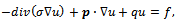 | (1) |
 | (2) |
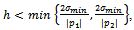
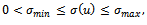 uniformly in u; in addition, q(x,y) ≥ qmin ≥ 0;(iii) for fixed (x,y)∈R, the function σ(u) satisfies Lipschitz condition in u with constant Γ (uniformly in x, y), Γ > 0.The nonlinearity introduced by the u-dependence of the coefficient σ(u) requires that, in general, the solution of equation (1) is approximated by numerical methods.We superimpose on R∪∂R a grid of points Rh∪∂Rh; the set of the internal points Rh of the grid are the mesh points
 , for i = 1, ..., N and j = 1, ..., M, with uniform mesh size h along x and y directions respectively, i.e.
  and
and  for i = 0, ..., N, j = 0, ..., M.Thus, at the mesh points of R∪∂R,
  for i = 0, ..., N+1, j = 0, ..., M+1, the solution
  is approximated by a grid function
  defined on Rh∪∂Rh and satisfying the boundary condition (2) on ∂Rh.In order to approximate partial derivatives in (1) we shall make use of difference quotients of grid functions. The forward, backward and centered difference quotients with respect to x and to y of the grid function
  at the mesh point
 , are, respectively:
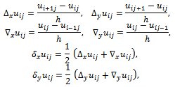 while the centered second difference quotient with respect to x and to y can be written
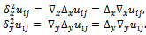 This notation was introduced by Courant et al. in[4].Providing a discretization error O(h2), the finite difference approximation of (1) in
  , i = 1, ..., N, j = 1, ..., M, is given by
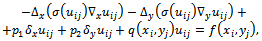 | (3) |
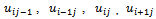
 , (i.e., l=(j-1)•N+i with j = 1, ..., M, and i = 1, ..., N), we can write the vector u of components
  and the difference equations (3) as the nonlinear system
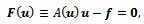 | (4) |
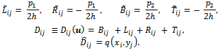
 respectively, are
 , and
, and , where
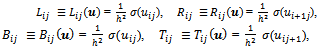 | (5) |
 | (6) |
 | (7) |
 ) or irreducibly (when
 ) diagonally dominant ([24, p. 23]) and has positive diagonal elements,
  r = 1, ..., n, and nonpositive off diagonal elements
 with r,s = 1, ..., n; therefore A(u) is an
  -matrix ([24, p. 91] or[18, p. 110]).In the case of diffusion equation
  , the matrix A(u) is also symmetric; then it is a symmetric and positive definite matrix ([24, p. 91]).The vector f in (4) has components
  for i = 1, ..., N, j = 1, ..., M and l = (j-1) • N+i.We remark that while the grid function
  is defined on the whole mesh region Rh∪∂Rh, the vector
  represents the grid function
  defined only on the interior mesh points Rh.Here, we suppose that a solution
  of the system (4) exists in
  (see Section 4).For solving the nonlinear system (4) the easiest and maybe the most common method is to lag the nonlinear term in (4) generating an iterative procedure denoted as Lagged Diffusivity Functional Iteration.With this iterative procedure the nonlinear system (4) can be solved via a sequence of systems of linear equations.Specifically, given a sequence of positive numbers
  such that
  as
as  and an initial estimate
  of the solution
  of the system (4), we generate a sequence of iterates
 with the following rule for the transition from a current iteration
  to the new iterate
 :● Find an approximate solution
  of the linear system
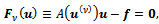 | (8) |
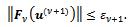 | (9) |
 and by an inner iterative solver of the linear system (8). This solver must be particularly well suited for implementation on parallel computers.The termination criterion for the outer iteration is provided by the following stopping rule
 | (10) |
 decreases as
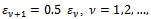 , with
 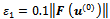 and
and  is a prespecified threshold.
3. Iterative Parallel Solution of the Linear Systems
- In this section, we remind the block form of the Alternating Group Explicit (AGE) and of the Arithmetic Mean methods for the solution of the linear system
 | (11) |
 | (12) |
 i = 1, ..., M, is a nonsingular NN matrix and the blocks
  and
and  (i = 1, ..., M;
  are square matrices of order N (n = N M).The AGE method consists in considering the following splitting of the matrix A
 where
where  and
and  are the following matrices
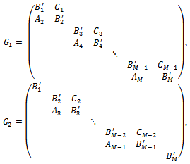 with
with Thus, starting from a vector
 , the AGE method generates a sequence of iterates
  as follows; for
  and k = 0, 1, ..., until convergence:
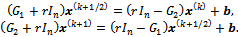 | (13) |
 is the identity matrix of order n. The AGE method is convergent when the matrices
  and
and  are symmetric and positive definite with
 . In this case it is proved that the optimal choice for r is
  where
where and
and , s = 1, 2, are the eigenvalues of the matrix
  (see, e.g.[1]).Furthermore, if the matrix A is irreducibly (or strictly) diagonally dominant with positive diagonal elements,
  , and nonpositive off diagonal elements
 , and
, and | (14) |
 -matrix. Set
  and
and  s = 1, 2. The choice of r in (14) yields that the matrices
  are strictly (or irreducibly) diagonally dominant and have positive diagonal elements and nonpositive off diagonal elements, then
  are
are  -matrices with
  From the hypotheses on the matrix A, the matrices
  are nonnegative
 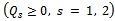 Thus, the iteration matrix T of the AGE method is
 Set
Set 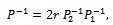 | (15) |
 (P is an
  -matrix) and
  holds. Indeed, set
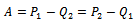 , a multiplicative splitting method can be written
 Then,
Then,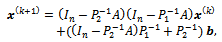 can be seen as a splitting method
 , i.e.,
  , by setting
 Since
Since , s = 1, 2, and
 , then we have the expression (15) for
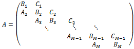
 .Now, the proof runs as that of the Regular Splitting Theorem in[18, p. 119].The Arithmetic Mean method uses the following two splittings of the matrix A
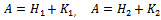 ,where
  and
and  are the following matrices
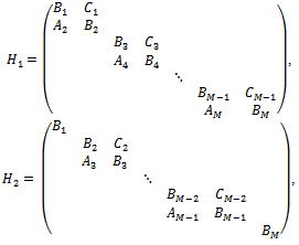 and
and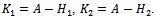 We suppose M even. If M is odd, we can proceed in a similar way.Thus, starting from a vector
 , the method of the Arithmetic Mean generates a sequence of iterates
  as follows; for
  and k = 0, 1, ..., until convergence:
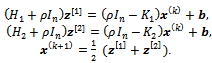 | (16) |
 ● positive definite but not symmetric with
  where
where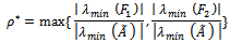 Here
Here  denotes an eigenvalue of a matrix V and
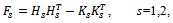 and
and  is the symmetric positive definite matrix
 ;● symmetric positive definite with
 At each iteration k of the AGE method, we have to solve M /2 linear systems of order 2N, i = 1, 3, 5, ..., M -1,
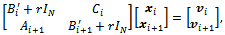 | (17) |
 . The solution of (17) can be seen as a block partitioned vector
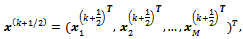 where each block has N components.Here
 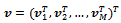 is the right hand side (r.h.s.) of the first equation of (13).These M / 2 systems can be solved simultaneously (in parallel).Then, in order to obtain the new iterate
  of the AGE method, we have to solve, in parallel, M / 2-1 systems as (17) with i = 2,4, 6, ..., M -2 and two linear systems of order N
 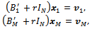 that can be solved in parallel, as well. The AGE method has an intrinsic parallelism.In the case of the additive splitting method of the Arithmetic Mean, at each iteration k we have to solve M-1 linear systems of order 2N, i = 1, 2, 3, ..., M -1,
 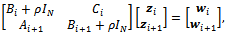 | (18) |
 and
and  indicate the vector
  (for i = 1, 3, 5, ..., M -1) and the corresponding r.h.s. of the first equation of (16) or the vector
  (for i = 2, 4, 6, ..., M -2) and the corresponding r.h.s. of the second equation of (16).Furthermore, we have to solve two linear systems of order N
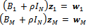 where
where  and
and  indicate the first and the last block of the vector
  and
and ,
,  the corresponding r.h.s. of the second equation of (16).These systems can be solved in parallel. The Arithmetic Mean method introduces also an explicit parallelism in order to increase the degree of multiprogramming, that is the number of processes that can be executed simultaneously ([13, p. 87]).When the system (11) arises from the finite difference discretization of the problem (1)-(2), the diagonal blocks of A in (12) are tridiagonal while the sub and superdiagonal blocks are diagonal.Thus, the systems (17) and (18) can be solved directly as in[9, 8] or iteratively, generating a two-stage iterative method as in[12]. A direct solution of these systems can be performed by cyclic reduction solvers ([17, p. 125],[15]) combined with an approximate Schur complement method ([17, p.123, p. 217]) or with block Gaussian elimination.
4. Analysis of the Convergence of the Lagged Diffusivity Functional Iteration Method
- In this section, we prove the convergence of the sequence
 generated by the lagged diffusivity iteration method for the solution of the system (4) under the smoothness assumptions (i)-(iii).We define
  and
and  i = 0, ..., N +1 and j = 0, ..., M +1, the grid functions defined on Rh∪∂Rh and satisfying the Dirichlet boundary condition on ∂Rh. For grid functions
  and
and  of this type, the discrete
  inner product and norm are defined by the formulas
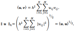 respectively.We say that the grid functions
  defined on Rh∪∂Rh and vanishing on ∂Rh satisfy Property A if they are uniformly bounded and have uniformly bounded backward difference quotients
  and
and  at each mesh point
  of Rh∪∂Rh. The set of all grid functions which satisfy Property A is denoted by
 . Thus,
  is the set of all grid functions
  for which there exist two positive constants
  and such that
  | (19) |
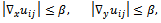 | (20) |
 is independent of h; also
  is independent of h but it depends on
  .(see[16]).We assume that the system (4),
  , where
 , has at least one solution
 .Suppose that the system (4) arises from the discretization of problem (1)-(2) subject to the conditions (i)-(iii) with
  and
and  being an irreducible nonsingular
  -matrix. If
  for any
 , then the mapping
  is uniformly monotone in
 . (See[16],[5] for a proof of this result and e.g.,[19, p. 141] for the definition of uniform monotonicity). The iterate
  of the lagged diffusivity functional iteration method satisfies the system (8) with the acceptability criterion (9), that is
  is the solution of the linear diffusion convection equation whose diffusivity depends on the previous iterate
  with inhomogeneous term
  We assume that all the iterates
  satisfy Property A. Thus in particular, by inequality (20), the backward difference quotients of each grid function are bounded and they depend on the inhomogeneous term; then, we have that there exist two constants
  and
and  such that
 | (21) |
 be a solution of the nonlinear system (4) with
 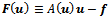 arising from the finite difference discretization of problem (1)-(2) subject to the conditions (i)-(iii) with
  and
and  being an irreducible nonsingular
  -matrix. Assume that the mapping
  is uniformly monotone in
 .Suppose that
  is a sequence of positive numbers such that
  as
as Let
Let  be arbitrary and let
  be the solution of
  satisfying the condition (9) with
  as in (8).If all the vectors
  belong to
  and satisfy Property A with (21) instead of (20), then the sequence
  converges to
  Proof. The proof runs as that in[6, Theor. 1] or in[5, Theor. 1, p. 33]. A more general result on the convergence of the lagged diffusivity functional iteration method can be obtained by defining the mapping u=G(u) where
 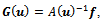 for all
 . A solution of the system (4) is a fixed point of the mapping
 . Since the smoothness condition (iii) on
 , we can have that the matrix A(u) satisfies the Lipschitz-continuity condition for every bounded subset
  of
of  with a Lipschitz constant
 Then we can write,
 Thus, we have for
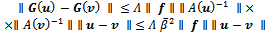 where
where  is a bound for
  for any
 . Here,
  indicates an arbitrary vector and matrix norm. The last inequality assures that the mapping
  satisfies a Lipschitz condition on a bounded subset
  of
of .
.5. Numerical Experiments
- In this section, we consider a numerical experimentation of the lagged diffusivity functional iteration method for the solution of the nonlinear system (4) generated by the finite difference discretization above described, of the elliptic problem (1)-(2). Indeed, we have to solve the system
 In these experiments, the vector solution
  is prefixed and it is composed by the values of the prescribed function
 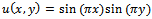 defined on the square
 The chosen functions for
  are
are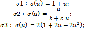 where, in the case of
 we have
  for a=3, b=2, c=1;
  for a=1.5, b=0.1, c=0.9 and
  for a=1, b=0.01, c=0.99.The vector
  is computed as
 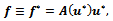 where the matrix
  of order n, has elements as in (5) and (6) with N=M and
 . In all the experiments we have N=256 and
  At each iteration
 of the lagged diffusivity procedure, we have to solve the linear system of order n
 with the splitting method of the Arithmetic Mean or of the Alternating Group Explicit described in a previous section (see e.g.[9],[10] for an evaluation of the block form of the Arithmetic Mean method on different parallel architectures and[7] for a description of the Fortran code implementing the method). These methods are compared with BiCG-STAB method implemented as in[14, p. 50].We call
  the new iteration of the lagged diffusivity procedure, computed with
  iterations of the inner solver such that the inner residual
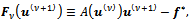 satisfies the condition (9)
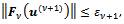 with
with 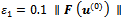 and
and | (22) |
 indicates the Euclidean norm. The vector
 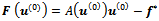 is the initial outer residual and its Euclidean norm is called
  The initial vector
  is taken as the null vector
  or as the vector e whose all the components are equal to 1
  .The lagged diffusivity procedure has been implemented in a Fortran code with machine precision
  and stops when (10) holds, i.e., for
 with
with  We call
  the iteration of the lagged diffusivity procedure for which condition (10) is satisfied. That is, the iterate
  satisfies
  (and we have
  and
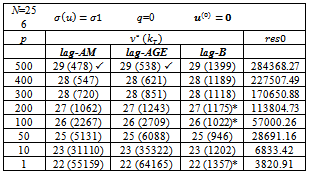
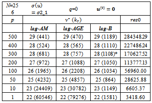
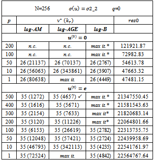
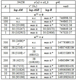
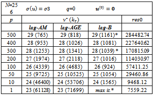
and In the tables, we report the number of iterations
  and, in brackets, the total number of iterations of the inner solver
 , i.e.,
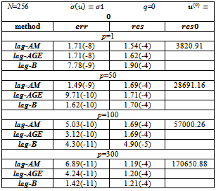
 In the tables, we also report the discrete
  norm of the error,
  the Euclidean norm of the outer residual
 and
and  The symbol * close to the value of res indicates that the behaviour of the norm of the outer residual
  is not monotone decreasing.The writing max it. indicates that at a certain iteration v, the maximum number of iterations of the inner solver has been reached. The maximum number of inner iterations is set equal to 20000.The writing n.c. indicates that at a certain iteration v, the condition (7) is not satisfied.The symbol " ü " close to the number of inner and outer iterations denotes that at a certain iteration v , the condition (7) is not satisfied and, in these cases, the lagged diffusivity iteration method generates the iteration by performing a prefixed number (equal to 20) of iterations of the inner iterative solver.The writing 1.71(-8) indicates
  In the tables, we indicate with lag-AM, lag-AGE and lag-B, the lagged diffusivity functional iteration method with the Arithmetic Mean, the Alternating Group Explicit and the BiCG-STAB method, respectively, as inner solver.Furthermore, we observe that, since
  decreases, for v increasing, as (22) and the lagged diffusivity functional iteration method stops at the iteration
  when the criterion for
  in (10) is satisfied, we have
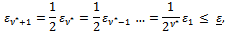 where we set
  Then,
Then, Indeed, in the experiments we obtain
|

|

|
 for
for 
|

|

|

|
6. Conclusions
- From the numerical experiments the following conclusions can be drawn:● the outer residual res has the same order of
 and the error err in the discrete
  norm has, in worst cases, order
 ● the AM method gives better results when the ratio between the maximum value of
  and the smallest component of
  is small, that is the coefficient matrix of the linear system is strongly asymmetric (see[20]) or the deviation from asymmetry is decreasing. We define as the deviation from asymmetry of a matrix the difference between the Frobenius norms of the symmetric and nonsymmetric parts of the matrix. Furthermore, we can observe the same behaviour of the AGE method with the one of the AM method, respect to the deviation from asymmetry of the coefficient matrix that occurs at each step of the lagged diffusivity procedure;● the lagged diffusivity functional iteration method combined with the AM or the AGE method breaks down when the coefficient matrix, at a certain iteration v , is not an
  -matrix (n.c.). In some cases, the AGE inner solver, requires a large number of inner iterations especially for nearly symmetric matrices;● the behaviour of the residual res when we use AM or AGE method as inner solver, is always monotone, except in one case where the lagged diffusivity procedure breaks down (the coefficient matrix is not an
  -matrix) but it has been possible to force the convergence by running a few number of iterations of the inner iterative solver. The nonmonotonicity of the residual happens at these "forced" iterations. This technique of forcing convergence is successful when condition (7) is "almost satisfied". ● the lagged diffusivity functional iteration method combined with the BiCG-STAB method, when it does not break down, requires a number of inner iterations that is not large and seems to be independent from the deviation from asymmetry of the coefficient matrix. We observe that the failure of the lagged diffusivity procedure with the BiCG-STAB method, in most cases, happens when the decreasing of the residual res is not monotone;● the behaviour of the lagged diffusivity procedure with AM or AGE method as iterative solver depends on the choice of the initial vector. The choice
  in the cases
  or
or  yields to negative values for
  for a certain v (tipically
  or
or  ) so that condition (7) is not satisfied; that is the initial iterate is too close to a region where a sufficient condition for determining the iterates of the outer procedure is not satisfied. Then, the control on condition (7) is a detection to start from another initial vector.