1. Introduction

There has been a global increase in harmful plankton blooms in last three decades[1-3]. Recently, there has been increasing interest in investigating the dynamics of harmful algal bloom (HAB) and its control[4 -7]. Plankton model is a kind of ecological model and different plankton models have been established and studied, previously[8, 9]. There are several papers in which attempts have been made to establish the role of different hydrological parameters in the formation of plankton blooms and then look for a suitable form of functional response to describe the reduction of zooplankton population due to toxin producing phytoplankton (TPP), for example, see[1, 2, 10, 11]. Reduction of grazing pressure of zooplankton due to release of toxic substances by phytoplankton is one of the most vital parameter in this context[12, 13]. Areas rich in some phytoplankton organisms e.g., Phaeocystis, Coscinodiscus, Rhizosolenia etc. are unaccepted/avoided by zooplankton due to dense concentration of phytoplankton or the production of some toxic as well as unpleasant factors by them and this phenomena is well explained by the exclusion principle[14, 15].

Buskey and Stockwell[16] have demonstrated in their field studies that micro and meso zooplankton population are reduced during the bloom of a chrysophyte Aureococcus nophagefferens in the southern Texas coast. These observations indicate that the toxic substance as well as toxic phytoplankton plays an important role on the growth of the zooplankton and have a great impact on phytoplankton zooplankton interactions. However, all the above studies do not explain several key features, such as, allelopathic interactions on the co-existence and persistence of phytoplankton species and its immediate effect on predators, control of recurring harmful algal bloom or oscillations and the effect of time lag required to release toxic substances.

In this stage, we would like to mention that various combinations of predational functional response and toxin liberation process give rise to several interesting dynamics of the system . In this study, we are mainly interested to present a mechanism for planktonic bloom in which the liberation of toxic substance or the effect of toxic phytoplankton is not an instantaneous process but is mediated by some time lag and can be helpful to reduce oscillations in the population and in turn, it is useful to maintain a stable co-existence of the species. The study of biological systems with time delays have been of considerable interest for a long time. There are also several reports that the zooplankton mortality due to the toxic phytoplankton bloom occurs after some time lapse (see, www.mote.org, www.mdsg.umd.edu). Our mathematical and field observations[17] also suggest that the abundance of Paracalanus (zooplankton) population reduces after some time lapse of the bloom of toxic phytoplankton Noctiluca scintillans and this allows us some considerable freedom for considering the delay factor in the model construction. Sarkar et al.[18] studied the role of two toxin producing plankton and their effect on phytoplankton zooplankton system. They considered the predational functional response as a linear and distribution of toxic substances as Holling type II functions. They suggested in this paper that the role of time lag and environmental fluctuations in the two harmful phytoplankton-zooplankton dynamics may give some interesting results and needs further investigation. Therefore, in this paper we have studied a mathematical model for a phytoplankton-zooplankton system considering both the Holling type II predational functional response and Holling type II functional form with time lag for the distribution of toxic substances.

2. Model Formulation and Basic Assumptions

The current study has been originated from the theoretical as well as experimental results on the interaction of harmful algal bloom and different types of phytoplankton zooplankton interactions[10, 16-20]. Motivated from the literature and the field observations[18, 20], a dynamical model consisting of two competing phytoplankton harmful to zooplankton has been proposed and the role of time lag in the underlying system is studied. Let P₁(t) and P₂(t) are the concentrations of the two kinds of harmful phytoplankton and Z(t) is the concentration of zooplankton at time t. Let r₁ and r₂ are the growth rates of the harmful phytoplankton, respectively, and k is the carrying capacity, which is assumed to be common for both the phytoplankton species. Let ρ₁ and ρ₂ are the rates of predation of both phytoplankton by zooplankton and γ₁ and γ₂ are the corresponding conversion rates of zooplankton, where the predator functional response is assumed to follow the Holling type-II functional response[21, 22], with h₁ and h₂ as half saturation constants. Let d is the natural death rate of zooplankton; α₁ and α₂ are the inhibitory effects of the two competing harmful phytoplankton. (γ₁ >) and (γ₂ >) are the rates of toxin liberation by the harmful phytoplankton reducing the growth of zooplankton. The discrete time lag τ is assumed to follow[23] and it is taken in the term describing the mortality of zooplankton due to liberation of toxic substances by two harmful phytoplankton P₁, P₂. The mathematical model is thus given by the following system of eSquations:

(1)

(2)

(3)

System of Equations (1)-(3) is supplemented with the following initial conditions:

3. Model Without Delay

(4)

(5)

(6)

3.1. Equlibria of the System

The equilibrium points of the system of Equations (4)-(6) are

1. The trivial equilibrium point: E_T ≡(0, 0, 0),

2. The axial equilibrium points: ≡ (0, k, 0)

and ≡ (k, 0, 0)

3. The boundary equilibrium points:

Where

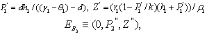Where

Now, we observe that the boundary equilibrium point exists if the inhibitory effects of both the harmful phytoplankton are less than certain thresholds, that is, if α₁< r₁/k, α₂< r₂/k. The equilibrium points and exist if d< (γ₁-θ₁) and d< (γ₂-θ₂).

4. The unique interior equilibrium point: ,

where

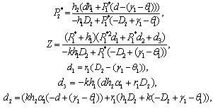The unique interior equilibrium point exist if

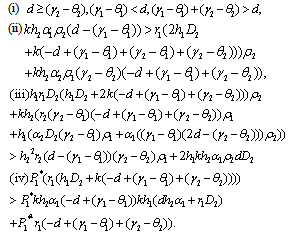
3.2. Dynamic Behaviour and Hopf-Bifurcation

Eigen value analysis to establish local asymptotic stability: By computing the variational matrix around the respective biological feasible equilibria, one can easily deduce the following lemmas:

Lemma 3.2.1 The steady state E_T (0, 0, 0) of system of Equations (4)-(6) is a saddle point.

Lemma 3.2.2 There exists two steady states (0, k, 0) and (k, 0, 0) which are feasible (one harmful phytoplankton and zooplankton free state) and are unstable saddle.

Lemma 3.2.3 There exists a zooplankton free steady state which is unstable saddle if

Lemma 3.2.4 There exists a steady state which is unstable if

Lemma 3.2.5 There exists a steady state which is unstable if

Next, we perform a stability study of the interior equilibrium point E*. For the sake of simplicity, the equilibrium point (,Z*) of the system of Equations (4)-(6) is shifted to a new point (x_1, x_2, x₃) through transformations

In terms of the new variables, the dynamical equations can be written in the matrix form as

(7)

where dot (.) over X denotes the derivative with respect to time. Here AX is the linear part of the system and B represents the non linear part. Moreover,

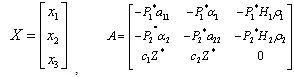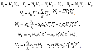
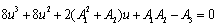
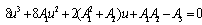
And

The characteristic equation of the community matrix corresponding to the linearized version of system of Equations (4)-(6) at E* is

(8)

Where

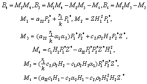
Using the Routh-Hurwitz criteria[22, 24], E* is locally asymptotically stable, if and . Here the conditions A₁ >0, A₃ >0 and A₁ A₂ >A₃ requires,

If one of the above mentioned conditions is violated then the system would become unstable around the positive interior equilibrium E*.

and (iii) the eigenvalues of the characteristic equation should be of the form λ_i = u_i+v_i, and, i=1, 2, 3. After substituting the values, the condition C = A₁A₂-A₃ becomes

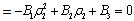(9)

The Equation (9) has at least one positive root say .

Therefore, one pair of eigen values of the characteristic Equation (8) at .are of the form , where v is positive real number.

Now, we will verify the Hopf-bifurcation condition (iii), putting λ_i = u_i+iv_i, in Equation (8), we get

(10)

On separating the real and imaginary parts and eliminating v between real and imaginary parts, we get

(11)

Again, differentiating (11) with respect to ρ₂, we have

Now, since at , we get

(12)

This ensures that the above system has a Hopf-bifurcation around the positive interior equilibrium E*. At the Hopf bifurcation point, where the real parts of complex conjugate eigen values are zero, the roots of Equation (8) are λ_1,2=±i v, λ₃=-A_1,

where v =│√A₂│and A₁ are to be evaluated at the bifurcation point.Next we seek a transformation matrix P which reduces the matrix A to the form

where the non-singular matrix P is given as

Where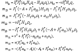

To achieve normal form of the Equation (7), we make another change of variable i.e. X =PY, where

Through some algebraic manipulations, Equation (7) takes the form

(13)

where, Ω = P^-1AP and

f is given by

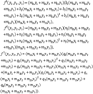Equation (13) is the normal form of Equation (7) from which the stability and direction of the Hopf bifurcation can be computed. In Equation (13), on the right hand side of the first term is linear and the second is non-linear in y’s. From these non-linear terms the stability and direction of the Hopf bifurcation is obtained[25].

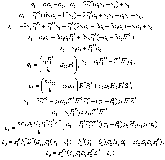
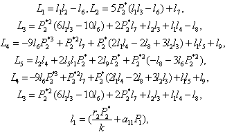
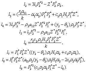
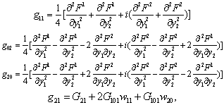where,

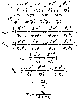All these partial derivatives are determined at the Hopf bifurcation point ρ₂ as well as at the origin. Based on the above analysis, we can see that each can be determined by the parameters. Thus we can compute the following quantities:

(14)

Theorem 3.1. μ₂ determines the direction of the Hopf bifurcation: if μ₂>0 (μ₂<0), then the Hopf bifurcation is supercritical (subcritical) and the bifurcating periodic solutions exist for ρ₂ > ρ₂* (ρ₂ < ρ₂*); β₂ determines the stability of bifurcating periodic solutions. and T₂ determines the period of the bifurcating periodic solutions, the period increases (decreases) if T₂ > 0 (T₂ < 0).

Now we will study the Hopf-bifurcation[25, 11, 26] of the system without delay taking ρ₁ as the bifurcation parameter. The necessary and sufficient conditions for the existence of the Hopf-bifurcation for ρ₁ = ρ₁*, if it exist are (i) A_i(ρ₁*) > 0, i=1, 2, 3 (ii) A₁(ρ₁*) A₂(ρ₁*) – A₃(ρ₁*) = 0 and (iii) the eigenvalues of the characteristic Equation should be of the form λ_i = u_i+iv_i, and, i=1, 2, 3. After substituting the values, the condition C = A₁A₂-A₃ becomes

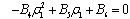(15)

Where,

The Equation (15) has at least one positive root say ρ₁ = ρ₁* Therefore, one pair of eigenvalues of the characteristic Equation (8) at ρ₁ = ρ₁* are of the form , where v is positive real number. Now, we will verify the Hopf-bifurcation condition (iii), putting λ = u+iv in (8), we get

(16)

On separating the real and imaginary parts and eliminating v between real and imaginary parts, we get

(17)

Again, differentiating (17) with respect to ρ₁, we have

Now, since at we get

This ensures that the above system has a Hopf-bifurcation around the positive interior equilibrium E*.

As above, similarly we have computed C₁(0), μ₂, β₂ and T₂ for studying the direction and stability of Hopf-bifurcating solution for the parameter ρ₁ and obtain,

(18)

Theorem 3.2. μ₂ determines the direction of the Hopf bifurcation: if μ₂>0 (μ₂<0), then the Hopf bifurcation is supercritical (subcritical) and the bifurcating periodic solutions exist for ρ₁ > ρ₁* (ρ₁ < ρ₁*); β₂ determines the stability of bifurcating periodic solutions. and T₂ determines the period of the bifurcating periodic solutions, the period increases (decreases) if T₂ > 0 (T₂ < 0).

Now we will study the Hopf-bifurcation[25, 11, 26] of the system without delay taking h₁ as the bifurcation parameter. The necessary and sufficient conditions for the existence of the Hopf-bifurcation for h₁ = , if it exist are (i) A_i()> 0, i=1, 2, 3 (ii) A₁()A₂()-A₃()= 0 and (iii) the eigenvalues of the characteristic equation should be of the form λ_i = u_i+iv_i and du/dh₁ ≠0, i=1, 2, 3. After substituting the values, the condition C = A₁A₂-A₃ becomes

(19)

Where,

The Equation (19) has at least one positive root say h₁ = Therefore, one pair of eigenvalues of the characteristic Equation (8) at h₁ = are of the form λ_1,2 = ≠± iv, where v is positive real number.

Now, we will verify the Hopf-bifurcation condition (iii), putting λ= u+iv in (8), we get

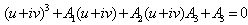(20)

On separating the real and imaginary parts and eliminating v between real and imaginary parts, we get

(21)

Again, differentiating (21) with respect to h₁, we have

Now, since at h₁ = , u(,) = 0 we get

This ensures that the above system has a Hopf-bifurcation around the positive interior equilibrium E*.

As above, similarly we have computed C₁(0), μ₂, β₂ and T₂ for studying the direction and stability of Hopf-bifurcating solution for the parameter h₁ and obtain,

(22)

Theorem 3.3. μ₂ determines the direction of the Hopf bifurcation: if μ₂>0 (μ₂<0), then the Hopf bifurcation is supercritical (subcritical) and the bifurcating periodic solutions exist for h₁ > (h₁ <); β₂ determines the stability of bifurcating periodic solutions. and T₂ determines the period of the bifurcating periodic solutions, the period increases (decreases) if T₂ > 0 (T₂ < 0).

Similarly if we take h₂ as the bifurcation parameter. The necessary and sufficient conditions for the existence of the Hopf-bifurcation for h₂ = h₂*, if it exist are (i)A_i(h₂* ) > 0, i=1, 2, 3 (ii) A₁(h₂*)A₂(h₂*)-A₃(h₂*) = 0 and (iii) the eigenvalues of the characteristic equation should be of the form λ_i = u_i +iv_i, and du/dh₂≠0, i=1, 2, 3. After substituting the values, the condition C = A₁A₂-A₃ becomes

(23)

Where,

The Equation (23) has at least one positive root say h₂ = h₂* .Therefore, one pair of eigenvalues of the characteristic Equation (8) at h₂ = h₂* are of the form λ _{1, 2} = ±iv, where v is positive real number and also

This ensures that the above system has a Hopf-bifurcation around the positive interior equilibrium E*.

As above, similarly we have computed C₁(0), μ₂, β₂ and T₂ for studying the direction and stability of Hopf-bifurcating solution for the parameter h₂ and obtain,

(24)

Theorem 3.4. μ₂ determines the direction of the Hopf bifurcation: if μ₂>0 (μ₂<0), then the Hopf bifurcation is supercritical (subcritical) and the bifurcating periodic solutions exist for h₂ > (h₂ <); β₂ determines the stability of bifurcating periodic solutions. and T₂ determines the period of the bifurcating periodic solutions, the period increases (decreases) if T₂ > 0 (T₂ < 0).

4. Stability of the Interior Equilibrium and Local Hopf Bifurcations of the Model with Time Delay

From the previous analysis we know that this system has seven equilibriums with certain conditions. In this section, we shall study the stability of the interior equilibrium and the existence of local Hopf bifurcations because the remaining six equilibria do not show the effects of delay in the analysis process.The characteristic equation of system of Equations (1)-(3) at the equilibrium E^* is

(25)

Where,

For stability of E^*, all the eigenvalues of the characteristic Equation (25) should have negative real part. It is difficult to analyze the condition under which Equation (25) has all roots with negative real part. However, for zero time delay, Equation (25) becomes

(26)

By Routh-Hurwitz criterion

(H1) then all roots of Equation (26) have negative real parts. Obviously, iw(τ )(w > 0)is a root of Equation (26) if and only if

(27)

Separating the real and imaginary parts,

(28)

(29)

which leads to

(30)

where

Let x = w², then Equation (30) becomes

(31)

and

Lemma 4.1. For the polynomial Equation (31), we have the following results.

(1) If r < 0, then Equation (31) has at least one positive root.

(2) If r≥0 and≤ 0, then Equation (31) has no positive roots.

(3) If r≥0 and ∆>0, then Equation (31) has positive roots if and only if and

The proof of Lemma 4.1 is similar to that in the proof of Lemma 2.1 in[7], we therefore omit it here.

From Equation (28) and Equation (29), we obtain,

(32)

(33)

Lemma 4.2 Suppose that x₀ = w²₀. Then the sign of α (τ₀) is coincident with that of h (x₀).

Proof. Let λ= λ (τ) be the root of Equation (25). Substituting λ(τ) into Equation (25) and differentiating both side of Equation (25) with respect to τ, it follows that

Thus

From (28)-(30), we have

where . Notice that Λ > 0 and w₀ > 0, we conclude that sign=sign This proves the lemma.

Theorem 5.1 Suppose that (H1) is satisfied

(i) If r≥0 and ∆≤0, all roots of Equation (25) have negative real parts for all τ ≥0, and hence the equilibrium E* of system of Equations (1)-(3) is asymptotically stable for all τ ≥0.

(ii) If either r < 0 or r≥0 and ∆> 0, x₁* > 0 and h(x₁*)≤0 holds then the equilibrium E* of system of Equations (1)-(3) is asymptotically stable for all τ ε[0; τ ₀).

(iii) If all conditions as stated in (ii) and h^’(x₀) ≠0 hold, then system of Equation (1)-(3) undergoes a Hopf bifurcation at the equilibrium E*, when τ =τ_j, j = 0,1,2,…….

5. Numerical Results

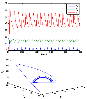
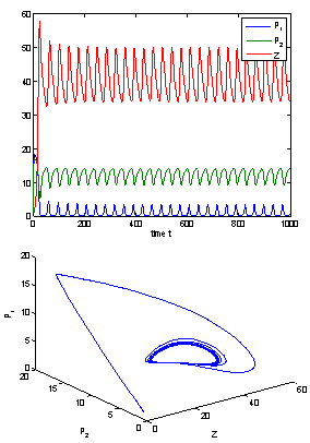
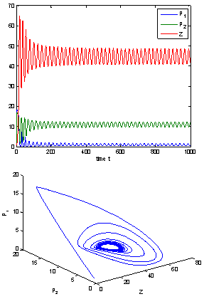
In this section we used MATLAB to perform some numerical simulation on system with delay and without delay. Firstly in the absence of time delay, we took some parameter values as

r₁ = 2.5; r₂ = 2.55, k = 20, α₁= 0.01; ρ₁ = 0.66; α₂= 0.02; ρ₂ =0.55; γ₁ = 0.43; γ₂ = 0.21; d = 0.1; h₁ = 12; h₂ = 10.8; = 0.09; = 0.06.

For this set of parameter values we observed that the positive interior equilibrium is E*(0.9127, 11.0817, 44.5116) which is asymptotically stable (see Fig. 1).

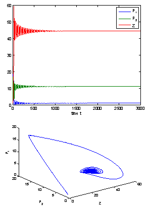Figure 1. The positive interior equilibrium point E*(0.9127, 11.0817, 44.5116) of system without delay is asymptotically stable

We studied the Hopf bifurcation of the system of Equations (4)-(6) taking ρ₂ as the bifurcation parameter, the transversality condition hold with these parameter when ρ₂= ρ₂* = 0:53106. Further, from the above process, we can determine the stability and direction of periodic solutions bifurcating from the positive equilibrium at the critical point ρ₂*. For instance, when

ρ₂= ρ₂* = 0.53106, C₁(0) = -0.0000269059-0.000139517i, Re{λ (ρ₂*)}= -0.0841233.

It follows from (14) that μ₂ < 0 and β₂< 0. Therefore, the bifurcation takes place when ρ₂ crosses ρ₂* to the left (ρ₂<ρ₂*), and the corresponding periodic orbits are orbitally asymptotically stable, as depicted in Fig. 2 and Fig. 3.

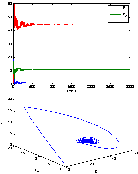
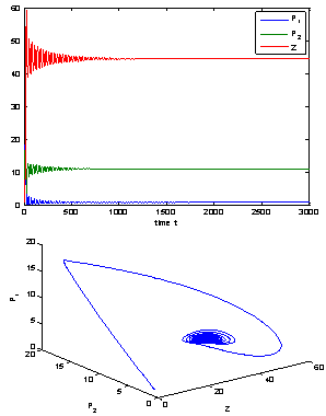
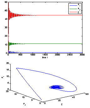Figure 2. The positive interior equilibrium point E* of system without delay is asymptotically stable when = 0.55 >= 0.531

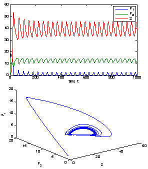
Figure 3. When= 0.4 < = 0.531, the positive interior equilibrium point E* of system without delay loses its stability and a Hopf-bifurcation occurs. Further, the bifurcating periodic solution is orbitally, asymptotically stable.

Further now take the value of ρ₂ = 0.55 > ρ₂*= 0.53106 then system of Equations (4)-(6) is stable, so we have studied the Hopf-bifurcation of the system of Equations (4)-(6) taking ρ₁ as the bifurcation parameter, the transversality condition hold with these parameter when ρ₁ = ρ₁* =0.683535. Further, from the above process, we can determine the stability and direction of periodic solutions bifurcating from the positive equilibrium at the critical point ρ₁*. For instance, when

ρ₁= ρ₁*= 0.683535, C₁(0) = -0.0000123894-0.000006.6961i, Re{λ¹(ρ₁*)}= 0.11223.

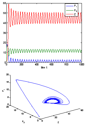
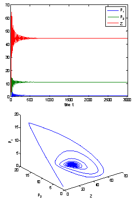
Figure 4. The positive interior equilibrium point E* of system without delay is asymptotically stable when = 0.66 <= 0.683535

Figure 5. When = 0.75 > = 0.683535, the positive interior equilibrium point E * of system (1) loses its stability and a Hopf-bifurcation occurs. Further, the bifurcating periodic solution is orbitally, asymptotically stable

It follows from (18) that μ₂ > 0 and β₂ < 0. Therefore, the bifurcation takes place when ρ₁ crosses ρ₁* to the right (ρ₁> ρ₁*), and the corresponding periodic orbits are orbitally asymptotically stable, as depicted in Fig. 4 and Fig. 5.

If we take ρ₁ =0.66 < ρ₁*= 0.683535 and ρ₂= 0.55 > ρ₂*= 0.53106 and taking h₁ as the bifurcation parameter, the transversality condition hold with these parameter when h₁ = = 11:7554. Further, from the above process, we can determine the stability and direction of periodic solutions bifurcating from the positive equilibrium at the critical point . For instance, when

h1 = = 11:7554, C₁₍0) =-0.00002467-0.0001229i, Re{λ^’()}= -0.0124335.

It follows from (22) that μ₂ < 0 and β₂ < 0. Therefore, the bifurcation takes place when h₁ crosse s to the left (h₁ <), and the corresponding periodic orbits are orbitally asymptotically stable, as depicted in Fig. 6 and Fig. 7.

If we take ρ₁=0.66< ρ₁*=0.683535, ρ₂=0.55> ρ₂*=0.53106 and h₁ =12> =11.7554, taking h₂ as the bifurcation parameter, the transversality condition hold with these parameter when h₂ = =11.2643. Further, from the above process, we can determine the stability and direction of periodic solutions bifurcating from the positive equilibrium at the critical point . For instance, when h₂ = = 11:2643, C₁(0) =-0.0000283042-0.000129115i, Re{λ ()}= = 0.00253856. It follows from (24) that μ₂ > 0 and β₂ < 0. Therefore, the bifurcation takes place when h₂ crosses to the right (h₂ > ), and the corresponding periodic orbits are orbitally asymptotically stable, as depicted in Fig. 8 and Fig. 9.

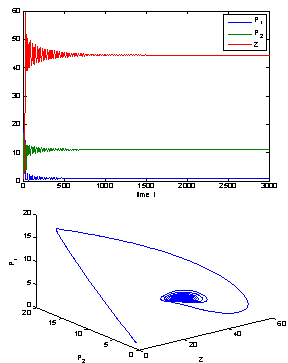Figure 6. The positive interior equilibrium point E* of system (1) is asymptotically stable when h1 = 12 >h1 * = 11:7554

Figure 7. When h1 =11< h1 * =11.7554, the positive interior equilibrium point E* of system (1) loses its stability and a Hopf-bifurcation occurs. Further, the bifurcating periodic solution is orbitally, asymptotically stable

Figure 8. The positive interior equilibrium point E* of system (1) is asymptotically stable when h2 = 10:8 > h2* =11.2643

Figure 9. When h2 =12>h2* =11.2643, the positive interior equilibrium point E* of system (1) loses its stability and a Hopf-bifurcation occurs. Further, the bifurcating periodic solution is orbitally, asymptotically stable

Figure 10. The positive interior equilibrium point E *of system (1) is asymptotically stable when = 9 < = 9.40825

Figure 11. When = 9.8 > = 9.40825, the positive interior equilibrium point E* of system (1) loses its stability and a Hopf-bifurcation occurs

If we take ρ₁= 0.66 < ρ₁*= 0.683535, ρ₂= 0.55 > = 0.53106, h₁ = 12 > = 11.7554, and h₂ = 10.8 < = 11.2643 the interior equilibrium point of the system becomes stable then we will study the role of time lag in the system. So we take delay as a bifurcation parameter and find out the critical value of delay parameter τ = τ₀ = 9.40825, the interior equilibrium point loses its its stability and Hopf-bifurcation occurs, as depicted in Fig. 10 and Fig. 11.

6. Discussion

In the previous studies, researchers have established with the help of experimental results and mathematical modeling that toxin-producing phytoplankton may be used as a controlling agent for the termination of planktonic bloom. But those studies do not contain the presence of two harmful phytoplankton in such situation. Moreover, the effect of time lags due to liberation of toxic substances and role of Holling-type II functional response cannot be ignored in this context. In this paper we have proposed and analyzed a three component model consisting of two competing harmful phytoplankton and a zooplankton. We have studied the stability behavior of the system around the feasible steady states. Our theoretical as well as numerical results show that for a certain threshold of the system parameters, the system possesses asymptotic stability around the positive interior equilibrium depicting the co-existence of all the three species. From qualitative and numerical analysis we find that ρ₁ and ρ₂ are bifurcating parameters for which the interior equilibrium point shows stable bifurcating solution when ρ₁ is greater than the threshold value and ρ₂ is less than the threshold value respectively. Similarly, we also find that h₁ and h₂ are bifurcating parameters for which the interior equilibrium point shows stable bifurcating solution when h₁ is less than the threshold value and h₂ is greater than the threshold value respectively. However, it is interesting to note that the dynamical nature of the bifurcating solution depends upon the parameters ρ₁, ρ₂, h₁ and h₂. When the time-lag is considered in the system, it is observed that the stable interior equilibrium point again exhibits Hopf-bifurcation for certain critical value of delay parameter.

ACKNOWLEDGEMENTS

Appreciation is extended toward the C. S. I. R., New Delhi, India, for their financial support, without which this research effort would not have been possible.