1. Introduction

The Allee model of growth has been widely and successfully used as a simple, yet adequate descriptor of the dynamics of small populations or critical depensation model[1], and many theoretical studies (e.g.[2],[3]) have been achieved. The Allee effect refers to reduced fitness or decline in population growth at low population densities. In population models, the Allee effect is often modeled as a threshold, below which there is population extinction.

In the present paper, we consider the Allee effect within the context of the symmetric model of three competing species. We wish to point out that an model of two competing species with Allee effect was proposed and studied in[2-4], and some papers dealing with experiments, simulations, or combinations of these competitive systems among others are described in[5-6]. In Section 2, we introduce the symmetric model of three competing species subject to the Allee effects. The main analytical results on stability analysis of the equilibrium points, are presented in Section 3. Section 4 is devoted to a discussion, in the context of numerical simulation, of the analytical results obtained in this paper. Concluding remarks on the paper are made at the end.

2. A three-species Competitive System Subject to the Allee Effects

In the three-species Lotka-Volterra competition models (e.g.[7-11]), it is possible for one- or two species extinction, or global stability of a positive three-species equilibrium, periodic solutions or a stable heteroclinic orbit (e.g.[12-14]). Here, we shall propose a new three-competitive model that specifically predicts Allee growth of speciesx,y, and z, respectively. Keeping this in mind, the model is described as follows:

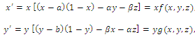(2.1)

,

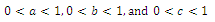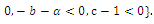
whereand z are the population densities, and are the quadratic intrinsic growth rates at intermediate densities, are the lower threshold of the population densities, respectively, and are the coefficients of interspecies competition, and (‘=. Throughout this paper we assume that .

In our model we consider that the intrinsic growth rates are quadratic and we prove that, under certain conditions, system (2.1) has at most twenty seven nonnegative equilibria. By using the software of MAPLE 10, a numerical example is provided to illustrate the behavior of the system (2.1) for a biologically reasonable range of parameters with only one asymptotically stable equilibrium point and seven unstable equilibrium points in. We believe that this is the first time that the three-species competition system (2.1) has been formulated and analyzed in the literature.

2.1. Boundedness of the Solutions

Consider the system (2.1). Obviously the functions are continuous and Lipschitzian with respect to all independent variables on. Therefore, a solution of the system (2.1) with nonnegative initial conditions exists and is unique. The basic existence and uniqueness theorem for differential equations ensures that

Lemma 2.1. The positive cone Int is invariant for system (2.1).

Lemma 2.2. The solutions of system (2.1) with positive initial conditions are bounded for all

Proof. Since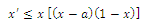, then. Here, we consider the case of strong Allee effect :

),

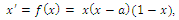where is the survival threshold. There are three equilibrium points . The relative extrema of the function are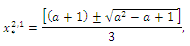

which give the points of inflection of the graph of versus t. The solutions are increasing and concave down when; increasing and concave up when decreasing and concave down when; decreasing and concave up when .We conclude that and are sinks; and is a source. Then if the initial population size is below a , the population will die out.

Similarly to and z , respectively.

3. Existence and Stability of Equilibrium Points

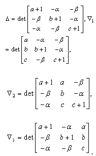
Computations of the boundary equilibria and the analysis of the existence of positive equilibrium points and their stability for system (2.1), provide the information needed to determine the coexistence or extinction of species. To do so, we compute the Jacobian matrix of (2.1). The signs of the real parts of the eigenvalues of evaluated at a given equilibrium point determine its stability. Here

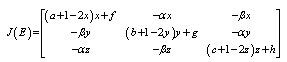(3.1)

where e are as in (2.1), , and all the parameters are positive. System (2.1) has at most twenty seven non-negative equilibria:

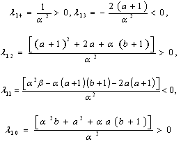
, with eigenvalues Thus, is locally asymptotically stable;

, with eigenvalues .This implies that is unstable;

, where eigenvalues. Thus, is locally asymptotically stable;

, where eigenvalues. This implies that is unstable;

, with eigenvalues. Thus, is locally asymptotically stable;

, where eigenvalues,. This implies that is unstable;

with eigenvalues Thus is locally asymptotically stable;

Now we establish criteria for the existence and stability of the equilibrium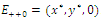. For this case, one of the three competitors goes to extinction depending on the initial values and the coexistence of three competing species described by (2.1) is not possible. Thus the exclusion principle holds[10].

When system (2.1) is restricted to, we obtain the following subsystem:

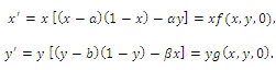(3.2)

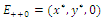An interior planar equilibrium occurring in the plane exists if and only if the algebraic system 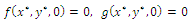has a positive solution. A routine computation yields

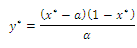and where

(3.3)

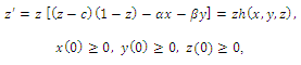
Using the rule of signs of Descartes it follows: (a) There are four sign changes in, so there are 4, 2 or 0 positive roots; (b) There are no sign changes at, so there are no negative roots. Hence, at most four positive equilibrium points are possible in the plane[15].

Under certain conditions on the parameters we have the following geometric interpretation (see Fig.3.1):

Proposition 3.1. Let 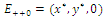denote an interior equilibrium in the plane. Then is the intersection of ellipses defined by

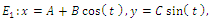(3.4)

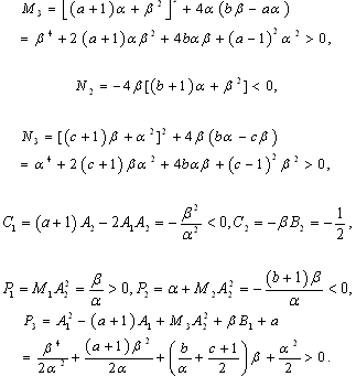
where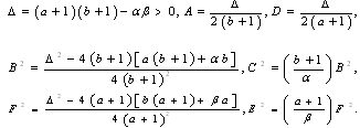

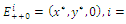
Proposition 3.2. Consider the system (2.1). Suppose that there are four interior equilibria in the plane; that is, Then only one equilibrium c of coexisting populations is locally stable and its basin of attraction is bounded by the stable separatrices of the saddle B s and D , both coming from the unstable node A.

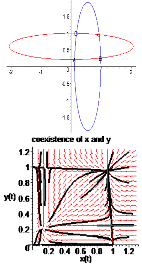Figure 3.1. Intersection between two ellipses. The equilibrium points are: is an unstable node; is a saddle point; is locally asymptotically stable; is a saddle point. Here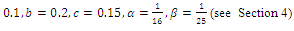

Similar results for the existence and stability of the equilibrium points and are obtained from (2.1).

3.1. Existence, Stability and Linearization of Positive Equilibrium Points

Let denote an interior equilibrium point of, if it exists. It follows from direct substitution and algebraic manipulation:

Proposition 3.3. System (2.1) has at most eight equilibrium points in the interior of. Their equilibrium values and are given by

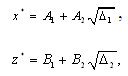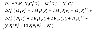
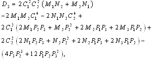
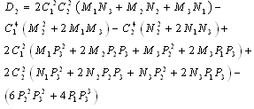
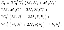
and is a positive root of

(3.5)

where

,

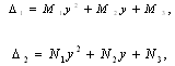
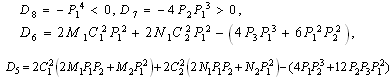
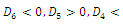
Corollary 3.1. Suppose that and Then has 8, 6, 4, 2 or 0 positive roots.

Corollary 3.2. Suppose Then has at least one positive root.

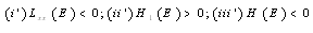
Proof. Clearly, and Hence, there exists a so that This completes the proof.

Remark 3.1 Using the software MAPLE, we obtain the following numerical examples:

(i) none positive equilibrium;

(ii) two positive equilibriums with eigenvalues (-,+,+),(+,+,+);

(iii) two positive equilibriums with eigenvalues (-,+,+),(+,αiβ), α;

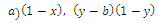
(iv) four positive equilibriums with eigenvalues (+,+,+),(+,-,+),(-,-,+),(-,+,+).

It is always informative to draw the set of positive equilibrium points of the system (2.1) in Here the set is defined by the intersection of the surfaces:

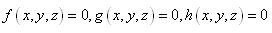(3.6)

Under certain conditions on the parameters of the system (2.1), we obtain (see Fig 3.2):

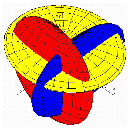Figure 3.2. Intersection between ellipsoids There are 8 equilibrium points in. Here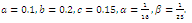

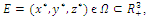
Proposition 3.4. Let denote the interior equilibrium of the system (2.1), if it exists. Then E is the intersection of three ellipsoids :

;

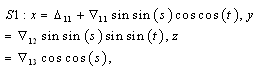
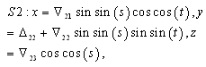
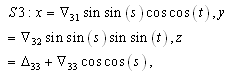
(3.7)

where

.

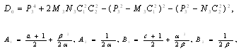
To determine the stability of a positive equilibrium point of (2.1), we will use the direct method of Lyapunov:

3.2. Direct Method of Lyapunov

Next let us consider the local stability of a positive equilibrium pointє, where is a neighborhood of to be determined. Based on the “direct method” of Lyapunov, we construct a continuous function

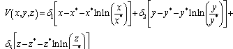(3.8)

where (i=1,2,3) are positive constant numbers which are yet unspecified, satisfying the following properties:

,

(b) 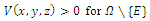, that is, the equilibrium point E is an isolated minimum of. In fact,

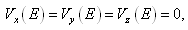
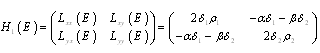
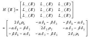
where the partial derivatives are calculated at.

(c) The function is continuously differentiable on the neighborhood, and, on this set, . Here,

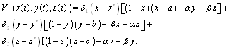Since, is a positive equilibrium point of system (2.1), satisfies

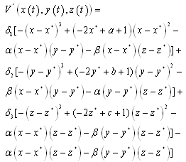(3.9)

If we prove that is an isolated maximum of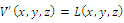, then (c) follows easily, that is:

(c1) We note that E is a critical point of the function that is

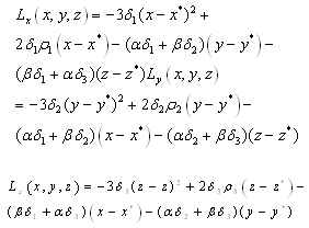implies.

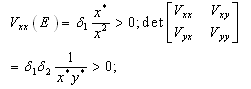
(c2) The equilibrium point E is a maximum point of

(3.10)

Here

;

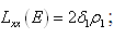
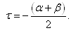
Letting we can rewrite (3.10) as

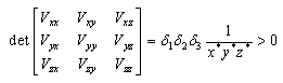
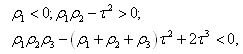
(3.11)

Thus, is a isolated maximum of, i.e., there is a neighborhood of such that, on this set . The pertinent result, which we prove, is the following (see Fig.3.3):.

Proposition 3.5. Consider the Lyapunov function (3.8) defined in the neighborhood of a positive equilibrium point E of the competitive system (2.1). If (3.11) occurs, then is locally asymptotically stable .

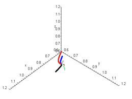Figure 3.3. Each graph depicts a three-dimensional population evolution in the state space for system. The initial conditions are (0,0,0),(0.9,0.9,0.9),(0.8,0.8,0.8),(0.7,0.7,0.7),(0.6,0.6,0.6),(1.0,0.9,0.9).The equilibrium pointis locally asymptotically stable. Here

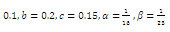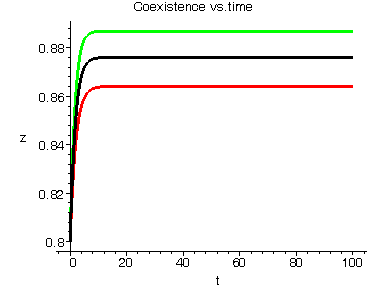Figure 3.4. Each graph depicts one-dimensional population changes with respect to time for system (2.1). Each trajectory starts at a point (0.8,0.8,0.8) near the equilibrium locally asymptotically stable: green-x , red-y, black-z. Here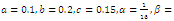

4. Numerical example

By using the software of MAPLE 10, a numerical example has been provided to illustrate the behavior of the system (2.1) for a biologically reasonable range of parameters. Choosing the following set of values for the parameters in (2.1):

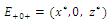
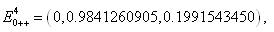
we find that the inequalities given by (3.11) hold for a unique positive equilibrium point and we observe that there are 27 equilibrium points given by

,

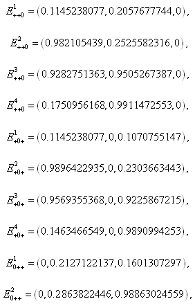
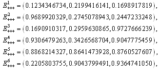
The of the positive equilibrium points (i=1…8) are roots of (3.5), that is, where

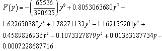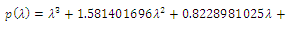
In the equilibrium point, the characteristic equation (4.11) of) reduces to, with roots.

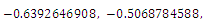
This implies that is a locally asymptotically stable equilibrium point. Here, we observe that the equilibrium points are unstable.

In the absence of a competitor, we have: (a) is a locally asymptotically stable equilibrium point, with eigenvalues -0.7346114284, -0.6340454548 and -0.2460382656. The equilibrium points are unstable. (b)is a locally asymptotically stable equilibrium point, with eigenvalues -0.7933441170, -0.6268358235, -0.2959390916. The equilibrium points are unstable. (c)is a locally asymptotically stable equilibrium point, with eigenvalues -0.7381379376, -0.5669278285, -0.1954752145. The equilibrium points are unstable.

In the absence of two competitors, we have: (d) is a locally asymptotically stable equilibrium point, with eigenvalues. The equilibrium is unstable. (e) is a locally asymptotically stable equilibrium point, with eigenvalues. The equilibrium is unstable. (f) is a locally asymptotically stable equilibrium point, with eigenvalues. The equilibrium is unstable.

Clearly is a locally asymptotically stable equilibrium point, with eigenvalues -0.1, -0.2, -0.15, respectively.

The of the equilibrium points (i=1…4) are roots of (3.3) . Intersection between two ellipses:

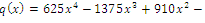
The of the equilibrium points. (i=1…4) are roots of. Intersection between two ellipses:

The equilibrium points are: is an unstable node; is a saddle point; is locally asymptotically stable; is a saddle point.

The of the equilibrium points (i=1…4) are roots of the polynomial:. Intersection between two ellipses:

The equilibrium points are: is an unstable node; is a saddle point; is locally asymptotically stable; is a saddle point.

5. Concluding Remarks

In this paper, a mathematical model of competition between three populations with lower threshold sizes has been proposed and investigated. The main focus was to analyze the question of existence and stability of nonnegative equilibria. Our results show that there exist at most twenty-seven equilibrium points for the system under consideration and, by using the software of MAPLE 10, a numerical example has been provided to illustrate the behavior of the system (2.1) for a biologically reasonable range of parameters with only one positive equilibrium asymptotically stable and 7 positive unstable equilibrium points.