1. Introduction

Modern process plants must be operated at high levels of availability in view of the huge cost of their installation, operation and maintenance. In this context, a reliability study should not only give an estimate of its availability, but also propose a means of discovering potential combinations of events which might result in catastrophic failures andevaluating the probabilities of their occurrence. The assessment procedure should be able to evaluate other performance measures and include cost-related aspects. Some of the important modeling approaches in reliability analysis are Network models, Fault Tree and Event Tree analysis (FTA and ETA), State-transition diagram and Petri Nets (PNs).

Network models are function-oriented. These models can tackle structural failures which lower the systemperformance. It is almost impossible to incorporate maintenance actions, software and human error and other cost-related aspects in network models.

Fault trees are event-oriented. The repair actions and the dependence between components cannot be easilyincorporated in the model. Standby redundancies, time-delayconditions and other dynamic behavior cannot be easily modeled using fault trees, since they are static in nature.

The biggest drawback of Markov models is the explosion of state space. Though it is possible to capture the dynamic behavior and dependence among components in this formulation, state-space explosion limits its usage. When formulating a Markov model of a complex system, it is difficult to ensure that all the possible combinations of events in a subsystem have been considered. Moreover, it is very difficult to use state-transition diagrams for model validation.

Out of network, FTA and Markov models, only FTA are widely used for safety and reliability studies of complex system since 1960s. The complete review of literature pertaining to FTA is provided in the reference[20]. However, FTA modeling approach is not useful for systems where components have interdependencies. The real-world systems will not comply to these requirements. Hence, there is a need for better modeling technique which can take care of real world complexities such as dependencies amongcomponents, modeling of repair actions, modeling of software and human related failures and events. Generalized Stochastic Petri Nets (GSPNs) are well suitable and could take care of these complexities in their modeling and gaining acceptance from research to industrial applications[21].

In this study, we employ Generalized Stochastic Petri Net, a graphical and mathematical modeling tool is used for studying a complex system, which is concurrent,asynchronous, distributed, parallel and nondeterministic. The use of Petri Nets for reliability analysis simplifies the task of the modeler considerably. It involves drawing a net representing a model of the system and marking it with the corresponding firing times of the transitions. If algorithms to construct the set of all reachable markings of a PN were available and if tools to automate the process of finding the probability of the markings could be built, then the analyst can concentrate more on reliability issues instead of writing and solving the equations for the underlying stochastic process. A systems approach is possible with PNs since hardware, software and human behavior can be modeled using the same language. It is also possible to incorporate safety and fault tolerance requirements.

2. Petri Nets

As per[1],[2],[3] and[4], Petri Nets have, over the last four decades, attracted the attention of researchers in several areas ranging from computer science to social sciences. PN can be introduced either algebraically or graphically. They are defined algebraically in terms of the following elements.

A PN is a 5-tuple, PN = (P, T, A, W, M₀), where

P = {P_1, P₂ ..., P_m } is a finite set of places

T = { t_1, t_2, ..., t_n } is a finite set of transitions

A ⊆ (P X T) U (T X P) is a set of arcs,

W is a weight function that takes values 1,2,3,... and

M₀ is the initial marking.

A standard PN consists of a set of "places" P drawn as circles, a set of "transitions" T drawn as bars and a set of directed arcs A. An arc connects a transition to a place or a place to a transition. Place may contain "tokens", which are shown as dots. The "marking" or the state of a PN is defined by the number of tokens contained in each place and is denoted by M. The construction of a PN model requires the specification of the "initial marking" M₀.

A place is called an "input place" to a transition if an arc exists from it to the transition. A place is an "output place" if an arc exists from a transition to the place. A transition is said to be "enabled" when all its input places contain at least one token. If the enabled transition is "fired", it removes one token from each input place and deposits one token in each output place. The firing of a transition modifies the distribution of tokens in places and thus produces a new marking for the PN.

For a given initial marking M₀ , the "reachability set" S is defined as the set of all markings that can be reached from M₀ by a sequence of transition firings. As per reference[8] and[9], in a Stochastic Petri Net (SPN), the firing time is an exponentially distributed random variable. Thus the marking sequence in a SPN obtained from the firings, is isomorphic to a continuous time Markov Chain. As per[7], in a Generalized Stochastic Petri Net (GSPN), the transition firing rates can be instantaneous or random firing time based on some distribution. Therefore the set of transitions can bepartitioned into a set of random timed transitions (with finite firing rate) and a set of immediate transitions. However, for any marking at which there are several enabled immediate transitions, a probability distribution must be specified, according to which firing of the transitions are selected.

3. System Modeling and Analysis

3.1. System Overview

The lubrication requirement for the combined cycle power plant is provided by a single lubricating oil system. A separate, enclosed, forced-feed lubrication module provides the lubricating and hydraulic oil requirements for the turbine power plant. This lubrication module, complete with tank, pumps, coolers, filters, valves and various control and protection devices, supplies oil to the gas turbine, steam turbine and generator bearings and accessory equipment. This oil absorbs the heat rejection from the bearings and shaft seal oil system. A portion of the pressurized fluid is diverted and filtered again for use as lift oil. The system is having more than 36 components. The system has to operate during start-up, normal operation, normal shut down and emergency shutdowns.

The following are the smaller subsystems associated with the lube oil system.

1. Lube oil tank assembly

2. Lube oil pump system

3. Lube oil cooler and filter assembly

4. Mist eliminator

5. Lift oil assembly

6. Lube oil clearance control

The construction of functional block diagram for the Lube oil subsystems as in Figure 1 is the first step towards its availability analysis. First, the components that can cause unavailability of each subsystem are identified. The reliability data for these components are taken from published sources and from the in-house records of the plant. Each component of the subsystem is considered to be in one of two states: good or complete failure.

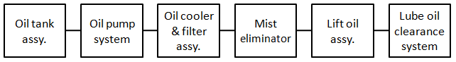Figure 1. Various subsystems in a Lube Oil System

The redundancies are taken into consideration in calculating subsystem reliability parameters such as MTBF and MTTR. The failure of a component may cause system failure depending upon the functional configuration of the system. A common-cause failure may also occur due to deficiency in equipment design, operation and/ormaintenance error and/or an external catastrophe.

3.2. Literature Review

The literature survey has revealed that Petri Net was considered as a powerful modeling tool and finds many applications in flexible manufacturing systems,communication protocols, computer hardware and software system. Reference[19] used Timed Petri Nets in modeling and analysis techniques to safety-critical real-time systems. These procedures allow safety, recoverability and fault tolerance. A hierarchical model for system reliability, maintainability and availability using GSPNs was proposed by[10]. Reference[11] proposed reliability models using timed Petri nets for a variety of fault-tolerant software, including mechanisms such as recovery blocks. The availability analysis of the core veneer manufacturing system in a plywood manufacturing system was performed by[16]. Reference[17] evaluated reliability parameters of a butter manufacturing system in a diary plant considering constant failure rates of various components. Semi-Markov processes and regenerative point technique are used to analyze three-unit standby system of water pumps in which two units are operative simultaneously and the third one is cold standby for an ash handling plant. The reliability and availability assessment of pod propulsion system using FMEA, FTA and Markov analysis is carried out by[18]. Reference[5] has analyzed pulping system using Petri Nets. The modeling and performance evaluation of thermal power plant using Markov approach is provided in reference[6].

Most of the models discussed in literature for estimating the availability and other reliability measures are based on the Markov approach and very few literatures are available for complex systems using Petri Nets. Reference[13] proposed a methodology based on Petri nets to evaluate the reliability parameters of a screening system in paper industry using GSPNs. The effects of failures and courses of action on the system performance have also been investigated.

This paper deals with the availability analysis of a Lube oil system used in a combined cycle power plant. The system is modeled as a Generalized Stochastic Petri Net (GSPN). The partial failures of the subsystems and common-cause failures are taken into consideration in the modeling and analysis and hence this research is more close to reality in modeling and analysis aspects.

4. GSPN Specification

The failure mechanism and repair process model of the lube oil system is given in Figure 2. The initial marking of the net contains tokens in the places P₀ to P₅ and P₁₉. This indicates that subsystems 0 to 5 are working initially. The token in the place P₁₉ indicates that the system is working normally. Tokens in the places P₀ and P₁₉ may enable the transition t₀, which corresponds to the partial failure of the subsystem 0. If the transition t₀ is fired, then it removes a token each from places P₀ and P₁₉ and deposits a token each in the places P₆ and P₁₇. The token in the place P₆ indicates the component 0 is in the partial failure mode and the one in the place P₁₇ indicates the system is in partial failed state. The token at P₆ can enable the transitions t_7, t_{8 or} t_9. The transition t₇ corresponds to the repair completion of the partial failed subsystem 0, whereas t₈ corresponds to the complete failure of component 0. If the transition t₇ fires then it removes a token each from the places P₆ and P₁₇ and deposits a token each in the places P₀ and P₁₉. This means that the component 0 is repaired and the system starts working normally. Suppose if the transition t₈ fires then it removes a token each from the places P₆ and P₁₇ and deposits a token each in the places P₁₂ and P₁₈. The presence of token in these places can enable the transition t_17. The repair action of the complete failure of the subsystem 0 is described by t_17. If the transition t₁₇ fires then it removes a token each from the places P₁₂ and P₁₈ and deposits a token each in the places P₀ and P₁₉. This means subsystem 0 is alright and the system is working normally. The common-cause failure of components 0 and 1 is described by the transition t_1. If the transition t₁ is fired, then it removes a token each from places P₀, P₁ and P₁₉ deposit a token each in the places P₁₄ and P₁₈. The common-cause repair action is depicted by the transition t_19. The failure and repair actions for the other subsystems are represented in a similar manner.

In this model the presence of a token in the place P₁₉ indicates that the system is in good state. Its complete failure is indicated by the presence of a token in the place P₁₈ and the partial failure of the system is indicated by the availability of the token in place P_17.

If,

T_o – is the mean time of a token is available in the places P_19.

T_r – is the mean time of a token is available in the places P₁₇ and

T_f – is the mean time of a token is available in the places P₁₈

Then, the availability of the Lube oil system is given by,

.

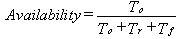Here, T_o is equivalent to the MTBF of the Lube oil system and (T_r + T_f ) is equivalent to its MTTR of the Lube oil system.

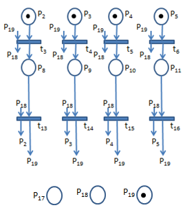Figure 2. GSPN Model of Lube Oil System

4.1. Generation of Reachability Tree

The first step in the analysis of PNs is the generation of the reachability tree. This is a set of markings that are possible from the initial marking. The nodes of the reachability tree represent the markings of the net, the root representing the initial marking. The directed edge from one marking to another indicates the firing of the corresponding transition. The analysis of the reachability tree will generate a lot of information about the system and a close examination enables verification of PN as a valid representation of the system being modeled. Thus, it is used for checking whether the model is a good representation of the system. The reachability tree is generated as follows.

Beginning with the initial marking, transitions which are enabled by this marking are identified and new markings that result from the firing of each of the enabled transitions are generated. Each new marking is added to the tree and the directed edges from the markings are drawn. The algorithm for generating the reachability tree is given below. The set of reachable markings along with its arc sets and reachability graph generated using the algorithm for the lube oil system are provided in Table 1, 2 and Figure 3. The entire algorithm is implemented in Excel and VBA.

m = total number of markings

i = 1 and m = 1

while i <= m do

for j = 1 to t do

if j is enabled by marking i then

generate new marking M_temp(k) and

for each k, do

if M_temp(k) is not already in the tree, then

m = m + 1

M_m = M_temp(k)

edge (M_i, M_m) = j

endif

endfor

endif

endfor

i = i + 1

endwhile

Table 1. The set of reachable markings Places Markings 0 1 2 3 4 5 6 7 8 9 10 0 1 1 1 1 1 1 0 0 0 0 0 1 0 1 1 1 1 1 1 0 0 0 0 2 0 0 1 1 1 1 0 0 0 0 0 3 1 0 1 1 1 1 0 1 0 0 0 4 1 1 0 1 1 1 0 0 1 0 0 5 1 1 1 0 1 1 0 0 0 1 0 6 1 1 1 1 0 1 0 0 0 0 1 7 1 1 1 1 1 0 0 0 0 0 0 8 0 1 1 1 1 1 0 0 0 0 0 9 0 0 1 1 1 1 0 0 0 0 0 10 1 0 1 1 1 1 0 0 0 0 0 11 0 0 1 1 1 1 0 0 0 0 0

Table 1. The set of reachable markings (cont.) Places Markings 11 12 13 14 15 16 17 18 19 0 0 0 0 0 0 0 0 0 1 1 0 0 0 0 0 0 1 0 0 2 0 0 0 1 0 0 0 1 0 3 0 0 0 0 0 0 1 0 0 4 0 0 0 0 0 0 0 1 0 5 0 0 0 0 0 0 0 1 0 6 0 0 0 0 0 0 0 1 0 7 1 0 0 0 0 0 0 1 0 8 0 1 0 0 0 0 0 1 0 9 0 0 1 0 0 0 0 1 0 10 0 0 0 0 1 0 0 1 0 11 0 0 0 0 0 1 0 1 0

Table 2. The set of arcs Start Marking End Marking Fired Transition 0 1 0 0 2 1 0 3 2 0 4 3 0 5 4 0 6 5 0 7 6 1 0 7 1 8 8 1 9 9 3 0 10 3 10 11 3 11 12 4 0 13 5 0 14 6 0 15 7 0 16 8 0 17 9 0 18 2 0 19 10 0 20 11 0 21

Figure 3. Reachability Graph

4.2. GSPN Simulation

At the beginning of the simulation run, the algorithm identifies all the enabled transitions from the initial marking. The firing time for each transition is determined by sampling from exponentially distributed firing intervals. The minimum firing time is selected and the corresponding transition is fired. The system moves to the next marking. The state of the system (good or complete failure) is ascertained. Failed subsystem, if any, will undergo repair. After repair the subsystem is as good as new. These events are simulated for thirty years. In order to reduce the standard deviation of the estimates of system down time and up time, a Variance Reduction Technique (VRT), viz., antithetic variate is used. The simulation is replicated a sufficient number of times to achieve convergence of results. The reliability data used in the simulation experimentation is given in the Table 3. The entire program is written using GPSS/H. The algorithm for the simulation is given below:

marking = initial marking

for j = 1 to t do

firing_time(j) = -1

while (simulation run not ended) do

for j = 1 to t do

if transition j is enabled, then

if firing_time(j) < 0 then

generate firing_interval

firing_time(j) = clock + firing_interval

endif

else (if not enabled)

firing_time(j) = -1

endif

endfor

find minimum firing_time(t)

fire transition t

reset firing_time(t) = -1

endwhile

Table 3. Reliability data used in this study Subsystem Partial Failure Rate (f/year) Full failure rate (f/year) Partial repair time (Hrs) Full repair time (Hrs) Tank assembly 0.0243 0.0486 3.5 7 Pump system 0.0478 0.0956 19.5 39 Cooler and filter 0.2856 5.5 Mist eliminator 0.3254 9.5 Lift oil 0.2041 8.5 Clearance control 0.0866 20 Common-cause failures 0.015 46

5. Results and Discussion

The results concerned with system down time, obtained from the simulation experiments are given in the Table 4. The first column is the replication number. The second column corresponds to simulation results using thetic random numbers and third column corresponds to simulation results using antithetic random number. The average value given in the 4^th column is finally considered as the simulation result of replication 1. Like this 30 replications are carried out to get steady state. The system availability graph is provided in the Figure 4. The system availability was found to be very high as 0.998825. It is estimated that 28.8 failures in 30 years.

Table 4. The thetic and anti-thetic simulation results of Lube oil system Replication # Thetic down time (Hrs) Anti-thetic down time (Hrs) Average down time (Hrs) 1 465.1 298.5 381.8 2 304.3 223.7 264 3 395.7 617.7 506.7 4 244.2 207.5 225.85 5 260.9 294.1 277.5 6 252.5 277.6 265.05 7 292.9 278.7 285.8 8 634 305.6 469.8 9 277.8 297.4 287.6 10 230.1 331.2 280.65 11 205.4 305.2 255.3 12 307.3 205.1 256.2 13 204.3 320.4 262.35 14 257.1 622.1 439.6 15 225.2 596.1 410.65 16 201.3 270.5 235.9 17 201.3 344.5 272.9 18 195.5 298.7 247.1 19 383.5 523.4 453.45 20 188.6 486 337.3 21 414.6 308.1 361.35 22 276.2 220.6 248.4 23 242.3 420.3 331.3 24 188.2 319 253.6 25 326 210.6 268.3 26 281.3 352 316.65 27 371.9 156.4 264.15 28 241.4 259.2 250.3 29 320.3 342 331.15 30 190.6 250.4 220.5

System downing events are calculated for various subsystems and the failure criticality indexes are assessed. These results are given in the Table 5 and Figure 5.

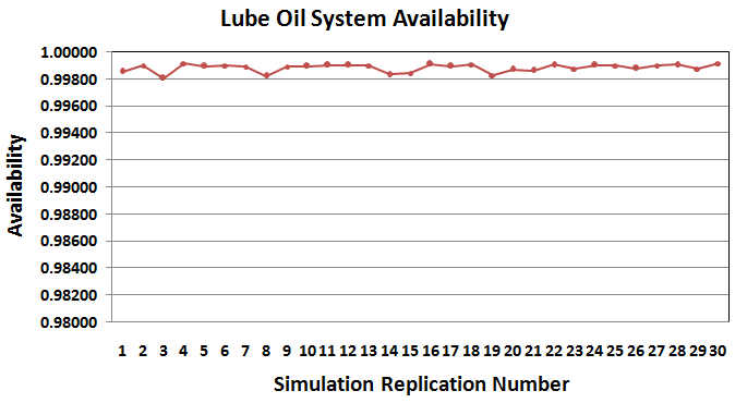Figure 4. The steady state system availability graph

We can now use the GSPN model to study the effects of the various component failure rates on the availability of the system. PCVs, DCV (components in Oil cooler and filter assembly) and pressure loss in the piping system were found to be major reasons for unavailability. The failure modes of PCVs are fails open and fails close. The major failure modes for DCV are struck and fail to seal. A close monitoring and maintenance actions are required to minimize these failures.

The proposed GSPN model has been successfully used for the estimation of the availability of the system. Any changes in the system configuration such as redundancy or replacement of a component by a more reliable one can easily be incorporated into the model and their effects analyzed. It is also possible to analyze the system when different maintenance strategies and repair policies are adopted.

Table 5. The various subsystems’ downing events and their failure criticality index Subsystem Failure Criticality Index System Downing Events Tank assy 0.028 0.8 Pump system 0.041 1.2 Cooler and filter 0.299 8.6 Mist eliminator 0.328 9.5 Lift oil 0.201 5.8 Clearance control 0.089 2.6

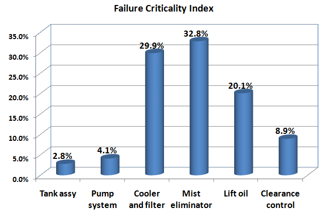Figure 5. The failure criticality index of various subsystem

6. Qualitative Comparison of Various Modeling Methods Used in Availability Studies

Modeling is the process of constructing a representation of a real-world system, reflecting its properties to the desired degree of detail. The model may be physical or abstract. Physical models are largely useful for purposes of teaching or training. Abstract models are useful in design, implementation and operations. These models bridge the gap between the real system and theoretical analysis. A number of modeling approaches such as network, fault tree, Markov and Petri Nets have been developed for the computation of reliability characteristics of complex technical systems. These models are either structure-oriented or event-oriented. The structure-oriented models allow us to tackle structural failures that cause undesirable deviation from the expected performance. Network models are the best examples for this category. Event-oriented ones can, not only model hardware failures but also model undesirable situations that may develop due to error in software, operation or maintenance. The nature of the problem, the objectives and the size play a vital role in selecting a model.

This study has been devoted to the estimation of reliability/availability of complex systems. Model, suitable for real-world complex problems, have been proposed. Despite a lot of earlier work in this field, there is a scarcity of methods to tackle a complex problem with all hardware and software failures, human errors and other dynamic features such as standby redundancies, repair actions and operator corrective actions. It is very difficult to accommodate repair actions and dynamic features into the network models. For complex systems, fault tree is used in the safety analysis for chemical / nuclear industry, is chosen as the tool for analysis. It is very difficult to include repair actions in the fault tree representation. The need for an analytical model in this context led to the Markovian approach. Markov models are capable of including all the real-world complexities, but the state space explosion limits its usage. Petri Net, a mathematical modeling tool, is adequate for the development of methodologies for prediction and evaluation of RMA of the system. GSPNs are used to find the availability of the lube oil system. This is an effective modeling tool which has immense potential for reliability studies. Using this, one can satisfy or at least try to satisfy all the reliability requirements.

7. Summary

The use of PNs for modeling complex systems for the purpose of availability assessment is demonstrated. The superiority of the GSPN over other approaches such as FTA and Markov models is brought out. The numerical estimates of the availability of the Lube oil system are obtained by simulating the GSPN. In this study the partial failure of subsystems and common-cause failures and repair actions are modeled using GSPN and analyzed. However, the modeling has the capability to incorporate software and human related failures and events. Thus, the proposed model can be conveniently used for modeling, analyzing and evaluating any complex stochastic systems.