Sugiono 1, Mian Hong Wu 2, Ilias Oraifige 2
1Department of Industrial Engineering, University of Brawijaya, Malang, East Java, Indonesia
2School of Technology, University of Derby, Derby, DE223AW, United Kingdom
Correspondence to: Sugiono , Department of Industrial Engineering, University of Brawijaya, Malang, East Java, Indonesia.
| Email: |  |
Copyright © 2012 Scientific & Academic Publishing. All Rights Reserved.
Abstract
Previous research works tried to optimize the architectures of Back Propagation Neural Networks (BPNN) in order to enhance their performance. However, the using of appropriate method to perform this task still needs expanding knowledge. The paper studies the effect and the benefit of using Taguchi method to optimize the architecture of BPNN car body design system. The paper started with literatures review to define factors and level of BPNN parameters for number of hidden layer, number of neurons, learning algorithm, and etc. Then the BPNN architecture is optimized by Taguchi method with Mean Square Error (MSE) indicator. The Signal to Noise (S/N) ratio, analysis of variance (ANOVA) and analysis of means (ANOM) have been employed to identify the Taguchi results. The optimal BPNN training has been used successfully to tackle uncertain of hidden layer’s parameters structure. It has faster iterations to reach the convergent condition and it has ten times better MSE achievement than NN machine expert. The paper still shows how to use the information of car body shapes, car speed, vibration, noise, and fuel consumption of the car body database in BPNN training and validation.
Keywords:
Genetic Algorithm, Neural Network, Car Body Design, Taguchi Method, MSE, Optimization, Back Propagation, Signal To Noise (S/N) Ratio, Analysis Of Variance (ANOVA), Analysis Of Means (ANOM)
1. Introduction
The back propagation neural network (BPNN) is widely used in industry, military, finance, etc. It is a tool to dealing with a system which very complex and difficult to obtain the mathematical model of the system. Literature review is used to see currently research direction and development in BPNN application. The commonly method to create the BPNN module is by the trial and error method. The method will be time consuming during the training procedure[1-3]. John F.C. Khaw and friends[4] investigated the optimal design of neural network using the Taguchi Method. They worked in NN’s parameters of number of hidden layer and number of node in hidden layer. The paper gives chance to study more NN’s parameters, e.g. transfer function, epoch, learning algorithm, parameter interaction, etc. Jorge Bardina and T. Rajkumar[5] studied the training data requirement for a neural network to predict aerodynamic coefficient. The paper shows manual NN training comparisons based on different transfer function and training dataset. It noted that dataset is important part to obtain a better MSE performance. Chien Yu Huang and friends[6] investigated the optimizing design of back propagation networks using genetic algorithm Copyright © 2012 Scientific & Academic Publishing. All Rights Reserved(GA) calibrated with the Taguchi method. They used Taguchi method successfully to define the GA parameters of population, mutation, cross over rate, and etc. Then the optimum GA is employed to optimize the NN training. In summary, complete and comprehensive BPNN investigation is needed to do better NN training process. As a result, parameters selection of multi layer perceptron (MLP) is still an open area for researcher. Genetic algorithm (GA) is commonly used to search the global optimum through the fitness functions by application of the principle of evolutionary biology and has been used for long time in different applications[7,8]. This paper shows how employ GA to adjust three learning algorithms; Conjugate Gradient(CG), Delta–Bar–Delta (DBD) and Quick Propagation for weights adjustment during the BPNN training.
2. Intelligent Car Body System Design
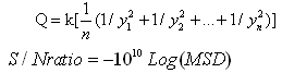
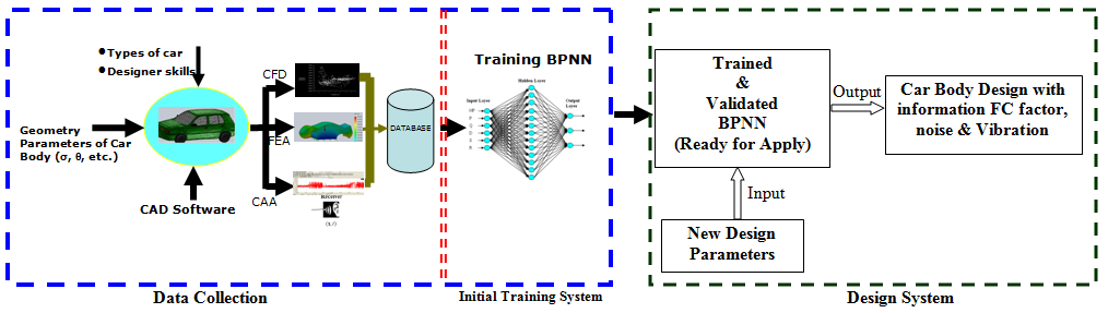
The Intelligent car body databases are employed to test the optimum BPNN architecture and to investigate the GA influence in the BPNN training performance. Figure 1 shows the developed intelligent car body design system in derby, UK. The system is divided into three sections included data collection, BPNN training section and design section. In data collect section, following data has to be collected and saved in database as: the information between car body geometry and fuel consumption, noise and vibration in varieties of speed, etc (table 1). In order to do it, the CAD, CFD, CAA and FEA software have been employed together to obtain the output information. The CAD (Computational Aided Design) software is used to create car body models in 3D view. The CFD (Computational Fluid Dynamic) is used to test the car models to get the information of fuel consuming factors (drag coefficient and lift force). The CAA (computational aeroacoustics) is used to test car models to get the information of noise (dB). Finally, the FEA (Finite Element Analysis) is used to test the car models to obtain the values of vibration in Z, X, Y, YZ and XY directions. At the end of the section, a database is ready to use by the next stage of BPNN training system.In the BPNN training system section, the optimum BPNN architecture has been trained by the data from the database. Taguchi tool is used to create the optimum BPNN architecture with 12 control variables (3 levels) and 3 noise variables (estate, hatchback and saloon car types). At the end of the second section, the optimum BPNN model is ready for application.Third section is new design application section which has completes all initial training tasks and the data collection tasks. In this section, the BPNN is ready to apply by user. User only needs to input the car body design parameters to the intelligent design system, a parameters based car body should be designed and with the full influence of vibration, noise and fuel consumption. As show the section two has employed the important tool of BPNN model, the following chart will give more details discussion on NNs.
3. Principle of Taguchi Method
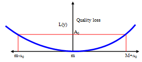
At the end of 1940, Dr. Genichi Taguchi offered new statistical approaches which have proven to be important tools in the design and process quality [9]. The Taguchi method is widely used in process design and product design that it is classified as “off line” of quality control. The Taguchi method is a technique for designing and performing experiments to optimise process design or product design where the system involves control factors, uncontrolled factors (noise factors), and interaction factors. The final design will be robust from a variety of multiple factors of signal input and signal noise. Orthogonal array (OA) is a special construction table in the Taguchi method to lay out the experiment. The OA is an experiment approach, which reduces the cost, improves the quality and enhances the robustness of a design. It is a matrix of numbers arranged in columns and rows that provides a set of well balanced, consistent and very easy experiments with a minimum number of factor combinations. The Taguchi method employs signal to noise (S/N) ratio and analysis of variance (ANOVA) to evaluate the best experiment design into amount of variability in the response and measurement of the effect of noise factors. They are also used to quantitatively determine the interaction between factors of an experimentThere are three Taguchi characteristics: a. minimum value, b. maximum value and c. nominal value. Each characteristic will be evaluated by different S/N approaches. The S/N ratio parameter analysis is set from electric analogy problem converted to logarithmic decibel scale. Signal-to-noise (S/N) ratio measures the positive quality contribution from controllable or design factors versus the negative quality contribution from uncontrollable or noise factors [9]. The following figure 2 and equations 1, 2, 3, 4 explain the quality loss function and S/N ratio.Quadratic loss function L(y) is defined in equation 1[10]: | (1) |
where: k = constant of quality loss function =  m = target valueLet y1, y2, y3, .., yn(yi is responses variable at i test), the average quality loss (Q) is given by equation 2:
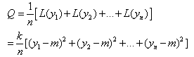 | (2) |
For the minimum criteria, m = 0: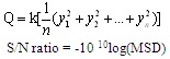 | (3) |
Where: MSD = Mean Square ErrorFor the maximum criteria, m = 
 | (4) |
Table 1. Input – Output Database for Saloon Car Body Design
 |
| |
|
 | Figure 1. Map of an intelligent car body design system |
 | Figure 2. Quadratic loss function in Taguchi method |
4. Optimum BPNN Architecture Car Body Design System
The optimum architecture of BPNN can be obtained by applying the Taguchi method. Figure 3 shows the steps of running the Taguchi method to optimize the BPNN architecture in the developed intelligence car body design system. The details of the description are in the following paragraphs.
4.1. Define the Taguchi Criteria
In the BPNN, controllable experiment factors of the Taguchi method include the number of neurons in each hidden layer, transfer function, number of hidden layers, epoch, etc. The response factor is the MSE of each BPNN training. Then the noise factor is defined in three different car body databases for estate, saloon and hatchback car types.
4.2. Identify Controllable Experiment Factors, Response and Noise Factors
In the BPNN, controllable experiment factors of the Taguchi method include the number of neurons each hidden layer, transfer function, number of hidden layer, epoch, etc. The response factor is MSE of each BPNN training. And then the noise factor is defined to be three difference car body databases for estate, saloon and hatchback car types.
4.3. Identify Levels and Experiments Factors
This step is to set up the details levels and values of the factors which are involved in building the optimum BPNN architecture. Table 2 shows an example for searching the optimum BPNN structure. It includes 8 factors which relate to the BPNN architecture parameters. They are defined from A to H. Three interaction factors are defined as A and (B or C), A and (D or E), (B or C) and (D or E). One error factor (I) is used in the table. There are three levels used in the table as well. The following paragraph will give the details of the explanation of the factors and interactions.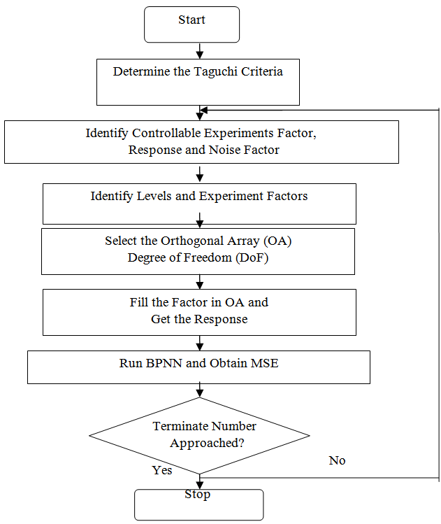 | Figure 3. Flowchart of Taguchi steps for optimization BPNN architecture in intelligence car body design system |
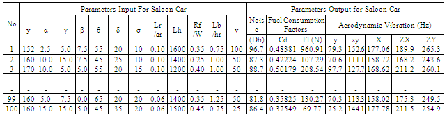
a. Number of hidden layers (A)MLP NN is formed by 3 different kinds of layers which are: input layer, hidden layer(s) and output layer. In general, one or two hidden layers are used by most research applications. As a result, values “1” or “2” can be chosen to hint the one or two hidden layer(s) structure.b. Number of neurons (B and C)The common used method to choose the number of neurons on hidden layer are defined by Kolmogorov’s and Lipmann’s[11] as follow:Lower bound of neurons in first hidden layer: | (4) |
Upper bound of neurons in first hidden layer: | (5) |
Lower bound of neurons in second hidden layer: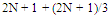 | (6) |
Upper bound of neurons in the second hidden layer :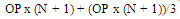 | (7) |
Where:N is the number of input neurons on the input layerOP is the number of neurons on the output layerThe Equations give the tolerance bend for user to select number of neurons. As a result, Taguchi method is used to define the optimum neurons in each layer. In table 2, the author gives the choice of number of neurons on each hidden layer. The number are calculated based on the information from car body database in table 1 which shows that the average input neurons are 8 and the average of output neurons are 8.c. Learning rules (G)Learning rules are used to define the weight value during the NN training. There are 3 learning rules used: conjugate gradient, Delta-Bar-Delta and quick propagation. All three rules are enhanced by applying the GA operation on them. The complete learning rules explanation and analysis is defined in section IV.d. Transfer function (D, E and F)The transfer function is used to squash the individual sum value of each neuron into the[-1, 1] range. Normally, each hidden layer employs the same Transfer function for its individual neurons. Five choices of the transfer functions are: Sigmoid, Tanh, linier Sigmoid, Linier Tanh and linier.e. Epoch set up (H)Epoch is the terminator condition. Here, the program will be terminated by the number of running cycle. It can be selected as 1.000, 5.000 or 10.000.f. Interaction factorsThe advantage of the Taguchi method is the author can investigate the existence of interaction between experiment factors. It determines whether the interaction is present, and a proper interpretation of the results is necessary. According to table 2, Three options of interaction factors that will be investigated are: A and (B or C), A and (D or E), (B or C) and (D or E).g. Error factor (I)The other advantage of the Taguchi method is the author can provide a place for the other NN factors that are not involved in the training process. The error factor could be contained momentum initial, learning rate initial, the other factor interactions, etc.
4.4. Select the Orthogonal Array (OA)
The Orthogonal Array (OA) has been categorised by Dr. Genichi Taguchi [65] into 2n series and 3n series array. They are named as L4 (23), L8 (27), L16(215), L32(231), L9(34), L18(21 x 37), L27(313), L36(313), etc. The OA is employed to screen all the experiment factors, levels, and responses. The Taguchi designs notation describes the OA lay out. It can be written as: Where: n = number of experimentP = number of levelk = number of column (factor)In this section one of the arrays should be selected for further application based on the calculation results of dof number of levels and number of factors. The dof is a measure of the amount of information that can be uniquely determined from a given set of data[12]. For a factor A with 3 levels, A1 data can be compared with A2 and A3. The n value in Taguchi design notation must be higher or the same value with the dof calculation based on experiment factors in table 2 above. The dof value is calculated by equation 8. It generated the total of dof as 27 as shown in equation 8a.
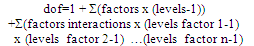 | (8) |
 | (8a) |
Table 2. BPNN’s Factors and Levels Configuration in Design of Experiment
 |
| |
|
Table 3. Standard Orthogonal Array L27(313) [9]
 |
| |
|
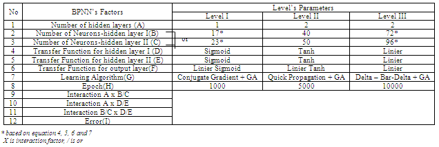
As a result, the best OA selection from the standard option is L27 (313) which is as table 3. Its design notation provides 13 factors of experiment, 3 level options for each factor and 27 parameters’ combinations.
4.5. Fill in the Orthogonal Array (OA) Table
In this step, the standard OA (table 3) is converted to OA for BPNN parameters (table 4) by filling factors of the experiment in appropriate columns of L27(313). The values and data used to fill in the table are stated as follows:Use standard OA L27 (313) table 3 to fill the factors of the experiment. According to table 2, there are eight main factors of experiment (A, B, C, D, E, F, G and H), three interaction factors (interaction between A and (B or C), interaction between A and (D or E), interaction between (B or C) and (D or E)) and one error factor.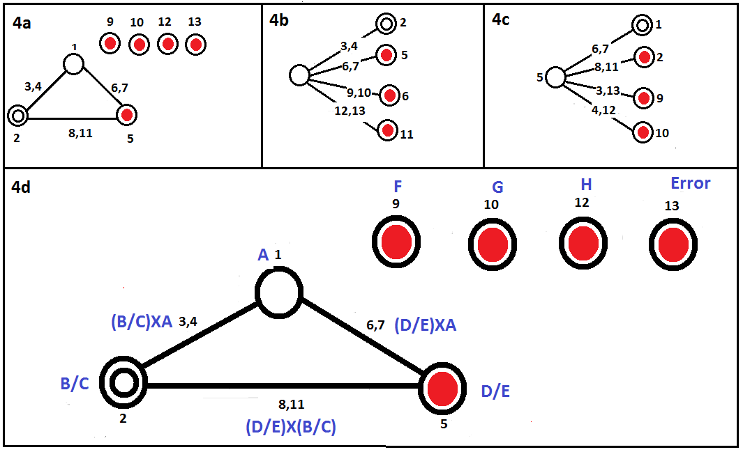 | Figure 4. a, b, c. Standard linier graph for L27 (313), d. the factors of the experiment are filled into the graph linier selected[9] |
Use a standard L27 (313) graph linier (Figure 4) to fill the factors of the experiment into a standard OA L27 (313) table. Linier graphs are used in Taguchi experimental design to allocate the appropriate columns of OA to the factors and interactions. There are three possible options of a standard L27 (313) linier graph as shown in figure 4a, b, c. According to main factors and interaction configuration, figure 4a is the best graph linier selection for 13 factors and 3 interactions. The circles are coded to place factors of experiment into OA’s column and the line between circles explains the factor of interaction. Point one points to a number of hidden layers (A factor). The number one should be a strong choice because, changing the number of hidden layers gives complex influence in mathematical description. Point two is used to B or C factor, point 5 is used to D or E factor, point 3 is placed at the interaction between A and B/C with leaved point 4 for nil (unused), point 9, 10 12, 13 are addressed to F, G, H, I factors randomly, etc.Convert the placement of factors of the experiment from linier graph in figure 4d into L27 (313) OA modification in table 4. According to the previous step, column 1 is for A factor, column 2 is for B and C factors, column 3 is for A to interact with B and C, etc. All OA codes in Table 3 work in 3 levels, except for A factor (number of hidden layer) which works in 2 levels (A1 and A2). The space for the third level is allocated to A2 as a dummy variable with the hypothesis (presumptive) that two hidden layers will provide a better performance than one hidden layer. As a result, OA’s code 1 in the A factor is replaced by A1 and OA’s code 2 is replaced by A2 respectively. Then OA’s code 1 in B/C factor is replaced by B1 for one hidden layer (A1) and B1C1 for two hidden layers (A2) and so on. The others factors of D/E, F, G, H, etc. will be treated in the same way.
4.6. Train the BPNN to Obtain MSE
In this stage, 27 BPNN structures have been created from Table 4. According to Taguchi method statistics, they are the best combination for conducting the experiments. The database (table 1) is used to train the BPNN individually and to get each MSE value of BPNN when they are met by the same terminate conditions. Each BPNN structure is tested three times for each car body type of saloon, estate and hatchback car. Then the average MSE values will be put into the BPNN results section of Table 4.
4.7. Taguchi Test Results Analysis
| Table 4. L27 (313) Orthogonal Array Modification for BPNN Parameters Optimization |
| | No | BPNN Parameters | BPNN Results | | A | B/C | (AXB)/C | NIL | D/E | (AXD)/E | NIL | (B/C) X (D/E) | F | G | NIL | H | I | Avg. MSE Saloon | Avg. MSE Estate | Avg. MSE Hatchback | | 1 | A1 | B1 | 1 | 1 | D1 | 1 | 1 | 1 | F1 | G1 | 1 | H1 | 1 | 0.02469 | 0.00771 | 0.00663 | | 2 | A1 | B1 | 1 | 1 | D2 | 2 | 2 | 2 | F2 | G2 | 2 | H2 | 2 | 0.02340 | 0.01857 | 0.02393 | | 3 | A1 | B1 | 1 | 1 | D3 | 3 | 3 | 3 | F3 | G3 | 3 | H3 | 3 | 0.02783 | 0.05135 | 0.05340 | | - | - | - | - | - | - | - | - | - | - | - | - | - | - | - | - | - | | 25 | A2 | C3B3 | 2 | 1 | D1E1 | 3 | 2 | 3 | F2 | G1 | 2 | H1 | 3 | 0.05657 | 0.06921 | 0.06915 | | 26 | A2 | C3B3 | 2 | 1 | D2E2 | 1 | 3 | 1 | F3 | G2 | 3 | H2 | 1 | 0.03691 | 0.02265 | 0.02808 | | 27 | A2 | C3B3 | 2 | 1 | D3E3 | 2 | 1 | 2 | F1 | G3 | 1 | H3 | 2 | 0.00753 | 0.00977 | 0.00847 |
|
|
| Table 5. S/N Ratios Results for Saloon Car |
| | Explanation | A | B | C | (AXB)/C | D | E | (AXD)/E | (B/C)X(D/E) | F | G | H | I | | Level 1 | 30.1 | 30.6 | 30.1 | 30.9 | 29.8 | 29.2 | 27.2 | 27.1 | 36.0 | 28.8 | 29.3 | 26.8 | | Level 2 | 28.3 | 27.5 | 26.6 | 29.7 | 30.8 | 31.1 | 29.9 | 31.0 | 25.7 | 31.1 | 29.7 | 31.8 | | Level 3 | | 28.7 | 29.0 | 27.9 | 26.9 | 26.1 | 30.0 | 29.3 | 30.2 | 27.4 | 27.8 | 29.3 | | Efect/Difference | 1.8 | 3.1 | 3.5 | 3.0 | 3.9 | 5.0 | 2.8 | 3.9 | 10.4 | 3.8 | 2.0 | 4.9 | | Rank | XII | VIII | VII | IX | V | II | X | IV | I | VI | XI | III | | Optimum | A1 | B1 | | | D2 | | | | F1 | G2 | H2 | |
|
|
Table 4 shows the input information and output MSE information for 27 different BPNN models. Next step of Taguchi method is to convert table 4 contents into S/N comparison table. To do so, the individual factor’s S/N should be calculated, e.g. Factor A1 in table 4 has 9 rows and they have the reporting MSE values, 0.02469, 0.02340, 0.02783, 0.03676, 0.01166, 0.03082, 0.03077, 0.05214 and then according to Eq. 3, S/N ratio for A1 should be calculated as: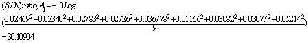 The S/N ratios table for estate and hatchback car have been investigated as well. Both of them have the same S/N ratios configuration. As a consequence, the optimum BPNN architecture used model A1-B1-D2-F1-G2-H2, same as the optimum BPNN architecture for a saloon car.The interaction effect is the one with the main effects of the factors assigned to the matrix column designed for interactions. According to table 5, the interaction between B/C and D/E gave MSE influence at 4th rank, the interaction between A and B/C gave MSE influence at 9th rank and interaction between A and D/E gave MSE influence at 10th rank. The calculation below shows one example of how to determine S/N ratio for interaction factors (A x B/C)1:
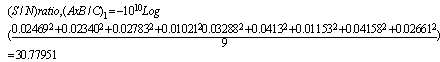 To determine whether two factors of experiment interact together, a proper interpretation of the results is necessary. The general approach is to separate the influence of interacting factors from the influence of the others. The interaction factors are analysed from the table 4. The interaction factor (A x B/C)1 is not the same as the factor (A1 x(B/C)1). In this analysis, the interaction columns are not used; instead columns of table 5 which represent the individual factors are used. The following example is a calculation of the interaction A1 x B1 based on mean analysis:A1 x B1 = (0.02469+0.02340+0.02783)/3 = 0.02531Figure 5 shows three interaction factors for the saloon car type. The complete explanation of the factors interaction is described below:The line A1 and A2 intersect. Hence, A and B/C interact.The line A1 and A2 intersect. Hence, A and D/E interact.The line B/C1, B/C2 and B/C3 intersect. Thus, B/C and D/E interact.By the same explanation, all the factors’ interaction’ in estate and hatchback cars are plotted intersecting with each other. It means that all factors have interacted significantly. Changing one interaction factor will influence the other factor interactions. The details percent of interaction impact in the BPNN performance are analysed by using the ANOVA approach.The analysis of variance (ANOVA) is the statistical treatment most commonly employed to analyse the results of an experiment to show the relative contribution of each factor experiment. The analysis of variance will be defined by the degree of freedom (dof), sums of square, mean square, F test, error, etc. Since the partial experiment is a simplification of the full experiment, the analysis of the partial experiment should be included in analysis of the confidence that it can be tackled by ANOVA. This research project employed two ways ANOVA which worked in more than one factor and three levels. The F test is used to determine whether a factor of experiment is significant relatively to the other factors in ANOVA table. Braspenning P.J and friends [11] classified F test range into three categories of:Ftest < 1: Section effect is insignificant (experimental error outweighs the control factor effect).Ftest ≈ 2: Section has only a moderate effect compared with experimental error.Ftest > 4: Section has a strong (clearly significant) effect.The ANOVA tables for estate and hatchback cars have been investigated as well. Generally, they have the same ANOVA configuration. The most influential is Factor F with 47.69 % in the estate car and 39.83 % in the hatchback car. Both error factors are smaller than in the saloon car with 3.13 % for the estate and 0.40 % for the hatchback car. Learning rule factors (G) in estate car and epoch factor (H) and interaction factor (AxD) in hatchback car are categorised as medium impact with percentages 5.70 %, 14.85 %, 8.52 % respectively put into medium impact.
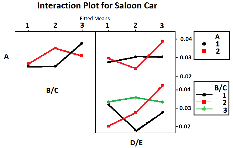 | Figure 5. Interaction plot for A x B/C, A x D/E, and B/C x D/E based on S/N ratios |
| Table 6. ANOVA Table of BPNN Parameters Effect for Saloon Car Type |
| | Factor | dof | SS | Adj. SS | MS | F- test | | Value | % | | A | 1 | 0.00001 | 0.00001 | 0.00001 | 0.05 | 0.14 | | A/B | 2 | 0.00025 | 0.00028 | 0.00014 | 0.51 | 2.50 | | D/E | 2 | 0.00047 | 0.00025 | 0.00013 | 0.45 | 4.64 | | F | 2 | 0.00519 | 0.00519 | 0.00260 | 9.32 | 51.50 | | G | 2 | 0.00053 | 0.00053 | 0.00026 | 0.94 | 5.21 | | H | 2 | 0.00005 | 0.00005 | 0.00002 | 0.08 | 0.45 | | I | 2 | 0.00088 | 0.00088 | 0.00044 | 1.59 | 8.77 | | A*(B/C) | 2 | 0.00030 | 0.00030 | 0.00015 | 0.53 | 2.94 | | A*(D/E) | 2 | 0.00021 | 0.00021 | 0.00011 | 0.38 | 2.10 | | (B/C)*(D/E) | 4 | 0.00080 | 0.00080 | 0.00020 | 0.72 | 7.94 | | Error | 5 | 0.00139 | 0.00139 | 0.00028 | | | Total | 26 | 0.01008 | |
|
|
After having completely investigated the Taguchi test results, the next step is to analyse the noise factor in the project. The noise factor has been defined as the types of the car body in the OA model. The investigation of noise contains analysis of mean difference and significant effect of noise factor in MSE performance and a t test must be employed as well. As we know, the t – test is a statistical test that is used to determine if there is a significant difference between the mean of two group data[12]. The following paragraphs explain: a. How to calculate t – test, b. Apply t test into noise analysis and c. t-test result.a. How to calculate t – testThe t- test is determined by involving the parameters of mean data, sample size and hypothesis mean as written in equation 9 and equation 10 below[14]. In this problem, the SPSS software is employed to calculate the t values. | (9) |
or | (10) |
where: n = sample size, n should less than 30. = mean data
 = hypothesis means = standard deviationSE = standard error meanb. Apply t test into noise analysisAs mentioned in OA table 4, the groups of MSE data are defined into three factor noise of estate, saloon and hatchback car types. The two tailed t – test is employed to measure whether or not three groups of MSE data are different to each other based on means analysis. There are three pairs of group data which should be investigated in t test between saloon – estate, between saloon – hatchback, and between estate – hatchback. The null hypothesis offers the author to accept ho and rejected h1 if the t-test value is smaller than the t-table standard or if significance 2-tailed value is bigger than 5% error α. The h0 has means that all three groups (saloon, estate and hatchback noise factor) are not significantly different in average mean; on the contrary h1 has means that all three groups are significantly different in average mean. The null hypothesis for the Taguchi test result is formulated as:
 and
and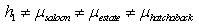 c. T test resultAccording to equation 9 and 10 and by using SPSS software, the t test result for paired difference data groups is shown in table 7. Based on the null hypothesis h0 and h1, the comparison between t test result and standard t table can be used to know the mean difference groups. It also used the comparison between Sig. (2 –tailed) from t test result and error α. All the group data comparisons are shown below:| t1 | > t0.5,v , so 1. 219 < 1.706 or Sig. (2-tailed) = 0.234 is bigger than 0.05| t2 | > t0.5,v , so 1. 538 < 1.706 or Sig. (2-tailed) = 0.136 is bigger than 0.05| t3 | > t0.5,v , so 0. 536 < 1.706 or Sig. (2-tailed) = 0.597 is bigger than 0.05Because all the t tests are smaller than t table or Sig. values bigger than α = 0.05, it is absolutely to accept h0 condition. It means that the noise factor (car databases) did not have a different set of data (MSE) configuration.
| Table 7. t-Test Table for Pair Data Sample |
| | Car Type Comparison | Paired Differences | t | dof | Sig. (2-tailed) | | Mean | Std. Deviation | Std. Error Mean | 95% Confidence Intervalof the Difference | | Lower | Upper | | Pair 1 | Saloon - Estate | 0.0043311 | 0.01846226 | 0.0035531 | -0.0029723 | 0.0116345 | 1.22 | 26 | 0.234 | | Pair 2 | Saloon - Hatchback | 0.0054389 | 0.01837174 | 0.0035356 | -0.0018287 | 0.0127065 | 1.54 | 26 | 0.136 | | Pair 3 | Estate - Hatchback | 0.0011078 | 0.01074398 | 0.0020677 | -0.0031424 | 0.005358 | 0.54 | 26 | 0.597 |
|
|
4.8. Conclusions of the Taguchi Result
In summary, the optimum BPNN parameters for all car types (saloon, estate and hatchback) are individually presented in Table 8 below. All the car types have the same optimum PBNN architecture. Moreover, all the interaction factors strongly interact with each other. The error factor (factor I) for saloon car is classified as moderate effect, but in contrast, factor I in estate and hatchback car is categorised as small impact.| Table 8. Summary of the Optimum BPNN Architecture |
| | No | Parameters | The Optimum BPNN Architecture | | Saloon Car | Estate & Hatc. Car | | 1 | A | 1 hidden layer | 1 hidden layer | | 2 | B | 17 neurons | 17 neurons | | 3 | C | - | - | | 4 | D | Tanh | Tanh | | 5 | E | - | - | | 6 | F | Linier Sigmoid | Linier Sigmoid | | 7 | G | Quick Prop + GA | Quick Prop + GA | | 8 | H | 5000 | 5000 | | 9 | A x (B/C) | Significant | Significant | | 10 | A x(D/E) | Significant | Significant | | 11 | (B/C) x (D/E) | Significant | Significant | | 12 | I | moderate | small |
|
|
4.9. Taguchi Verification
 | Figure 6. Taguchi verification for the optimum BPNN architecture in the intelligent car body design system |
The comparison between the optimum BPNN result and NN machine expert that people commonly use in “Neurosolution Software” has been used to verify the Taguchi results in the intelligent car body design system. All car types have been tested 10 times with different NN input data by using the optimum BPNN results and NN machine expert. The NN machine expert worked averagely at MSE = 0.03377, and the optimum BPNN architecture averagely worked at MSE = 0.00587. It means the new optimum BPNN architecture based on Taguchi optimisation improved the NN performance at around 82.62% from the current NN model. It can be inferred that the optimum BPNN architecture which is applied in the intelligent car body design system is much better than the current NN machine expert. Figure 6 shows this comparison for saloon, estate and hatchback car types.
5. Effect of GA in Training Performance
This section used to discuss the effective when the GA application in the intelligent car body design training is employed. According to table 2, the GA application is employed in the G factor of experiment as a method to adjust NN’s weights for all factors’ levels of learning rules. As a result, the NN training process worked in the optimum weights value selected. The discussion will divide into 4 steps for: 5.1. introduction the learning algorithm, 5.2. test BPNN without GA in intelligent car body training, 5.3. test BPNN with GA application in intelligent car body training, and 5.4. comparison the optimum BPNN training with or without GA application.
5.1. Introduction the Learning Algorithm in BPNN Weight Adjustment
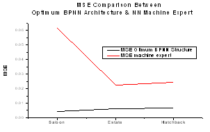
Learning algorithm is defined as a procedure for modifying or adjusting the weight on the connection of each of the neurons or units in the BPNN training process. The BPNN training involves 3 stages; the feedforward of the input training pattern, the calculation and backpropagation of the associated error, and the adjustment of the weight. In another side, learning rate and momentum are very important parameters in BPNN training process.The learning rate parameter in the first order gradient approach method is based on the step length. If the step size is too small, it will take too many steps to reach the minima (bottom) condition. Conversely, if the step size is too large, then it will approach the minimum point fast, but it will jump around the minimum point to left the large approach error. Figure 7 shows the impact of different step sizes to reach the optimum solution in weighting update. Approach step size is constant at Δl. So searching start from x0 and go through x1, x2 and the Δl will lead the net to jump over xmin point to x3. If the step length keeps at Δl, the searching result will be jumped at x3 and x2 point. | Figure 7. Effect of step size for achieving optima condition in NN training |
Momentum learning is a backpropogation parameter that can make the weight adjustment direction change to the opposite gradient direction occasionally, to avoid the approaching process from being trapped in the local optimum point. As a result, energy momentum can be employed to avoid the local optima of the learning process as was the case in the steepest decent algorithm. Energy momentum can be employed to avoid the local optima of learning process as was the case in the steepest decent algorithm. Energy momentum is defined as a function of momentum parameter ( ) time correction weight based previous gradient. The new weight has the ability to jump to the next searching while avoiding local minima (see figure 8). The convergence process is faster than steepest learning as an effect of using momentum energy. The momentum equation in backpropagation algorithm is presented by the new weight for training step t +1 based on the weight at training steps t and t -1. Momentum parameter has value in range from 0 to 1
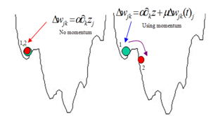 | Figure 8. Effect of momentum for achieving optimum condition in NN training |
Figure 9 chronologically explains the interconnection between BPNN and GA application to adjust weights parameter in the DBD learning rule. The activities in Figure 9 contains: collection and preparation of data, define robust (optimum) NN architectures, initialise population (connection weights and thresholds), assign input and output values to ANN, compute hidden layer values, compute output values, compute fitness using MSE formula. If the error is acceptable then go to the next step, but if it is not then go to next iteration of GA application and finally train the neural network with selected connection weights. The following part 5.2 and part 5.3 will show the Quick prop learning rate benefit in the optimum BPNN training for saloon, estate and hatchback car body databases.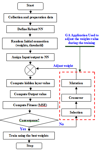 | Figure 9. Neuro-Genetic algorithm in BPNN development |
5.2. BPNN without GA in Intelligent Car Body Training
When the optimum BPNN structure has been designed, next step is to train the weight values in the BPNN. They are two training methods for this purpose: with or without GA support (fig. 10 & 11). The MSE values and convergence condition are used as indicators in the comparison test. The experiment parameters used Quick prop in initial learning rate = 0.50 and momentum = 0.0166. Figure 10 shows the iteration process of the optimum BPNN training without GA application for saloon car body database in 5 times running to ensure the stability of the results. According to the figure 10, the MSE training is convergence in epoch 5000. Finally, the BPNN training results gave average MSE performance for 0.04408686 in saloon car database.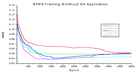 | Figure 10. BPNN training for saloon car without GA application |
5.3. BPNN with GA in Intelligent Car Body Training
The selection of connection weights in the neural network is a key issue in BPNN performance. The complex network connection will degrade BPNN performance to find the global minima. The randomisation method is commonly used to initialise the network weights before training. Genetic algorithm (GA) is employed to minimise fitness criteria (MSE) by BPNN weights adjustment. The main advantage of using GA is associated with its ability to automatically discover a new value of neural network parameters from the initial value. There are some GA parameters that are employed in this BPNN training:This study selected fitness convergence that the BPNN training will stop the evolution when the fitness is deemed as converged.The Roulette rule is employed to select the best chromosome based on proportionality to its rank.The initial values for learning rate and momentum are 0.500000 and 0.0166.Number of population is 50 chromosomes and generation number for maximum 100.Initial network weight factor is 0.1074.Mutation probability is 0.01.Using heuristic crossover.Crossover will combine two chromosomes (parents) to generate new chromosome (offspring). Green numeric indicates the best parent and red numeric is the worst parent. Below is an example of two parents that were used in the BPNN training.Parent 1: 11001010Parent 2: 00100111The heuristic uses the fitness values of the two parent chromosomes to determine the direction of the search. The offspring are generated according to the following equation 8[2]:Offspring1 = BestParent + r *(BestParent – WorstParent)(8)Offspring2 = BestParentThe symbol r is a random number between 0 and 1. One example of new chromosomes from parents 1 and 2 at r = 0.4 are:Offspring1 = (1+0.4(1-1) (1+0.4(1-1) (1+0.4(1-0)01010Offspring2 = 01000111orOffspring1 = (1)(1)(1.4)(0)(1)(0)(1)(0)Offspring2 = (0)(1)(0)(0)(0)(1)(1)(1)Figure 11 shows the MSE training process by the optimum BPNN architecture in five times simulation running. The saloon’s training gave an average of MSE = 0.004468267.
5.4. Comparison of the Optimum BPNN Training with or without GA Application
Figure 12 shows the comparison between the optimum BPNN training performance without GA application as explained in part B and the optimum BPNN training performance with GA application as explained in part C. The figure shows that by using GA, the optimum BPNN training has faster iteration to reach the convergent condition. It also has ten times better MSE achievement than the optimum BPNN training without GA application. In short, it can beconfidently said that the GA application could significantly increase the BPNN performance.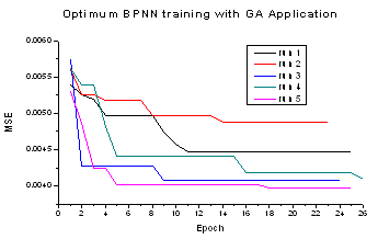 | Figure 11. NN training for saloon car with GA application |
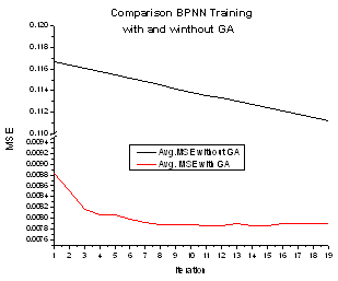 | Figure 12. Comparison of the optimum BPNN training with and without GA application |
6. Conclusions
In this paper, the Taguchi method for finding the optimum BPNN structure based car body design has been developed successfully. As example one of ten tests, design a saloon car body with the input parameters: y = 165 mm, α = 11°, γ = 12°, β = 7°, θ = 62°, δ = 21°, σ = 12°, Lr/ar = 0.01, Lh = 1525 mm, Rf/W = 0.90 and v = 90 mph is tested by two difference methods gave list of output as follow:List output based on BPNN module:• drag coefficient = 0.2056• lift force = 692.5 N• noise = 94.11 dB• vibration at Z = 491.07 Hz, at Y = 526.70 Hz, at YZ = 623.50 Hz, at X = 762.94 Hz, and at XY = 786.89 Hz.List output based on conventional (CFD, CAA and FEA ) test:• drag coefficient = 0.21541• lift force = 693.88 N• noise = 90.21 dB• vibration at Z = 493.05 Hz, at Y = 536.05 Hz, at YZ = 637.09 Hz, at X = 745.33 Hz, and at XY = 889.03 HzAccording to test results, the BPNN module can replace conventional method confidently.Many advantages can be obtained from using the Taguchi method. Firstly, authors enable to evaluate the impact of BPNN’s parameters including parameters’ interaction in the MSE performance. Transfer function in the output layer dominated the BPNN training performance with 51.50% for saloon car, 47.69% for estate car and 39.83% for hatchback car; no researchers investigated and founded it before. Secondly, the authors concluded that the car’s database is immune from the noise factor of car types as has been investigated by statistics approaches. Thirdly, there is strong interaction between number of hidden layer – number of neuron, number of hidden layer – transfer function and between number of neuron – transfer function in BPNN training. Fourthly, GA application in BPNN training can speed up the convergence condition and ten times increase the MSE performance. Lastly, it is a big chance to develop a software combination between NN parameters and design of experiment (DoE) – Taguchi tool adaptable with any databases. It will not only work in intelligent car body design system but it also can be used in any kinds of problems.
ACKNOWLEDGEMENTS
Thankful to the University of Derby, UK for supporting this paper.The authors are also grateful to the Ministry of National Education of the Republic of Indonesia and the University of Brawijaya, Malang Indonesia for their extraordinary courage.
APPENDIX
The ANOVA’s steps for a saloon car are calculated as follows:1. total of all results (T):T=0. 02469+0.02340 + 0.02726 + … + 0.00753= 0. 823462. correction factor (C.F.):C.F. = T2/n = (0.82346)2 / 27 = 0.02511, n = number of experiment, 27.3. total Sum of Square (SST):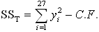 = (0. 024692+0.023402+0.027262+…+0.007532)-0.02511= 0.01008394. factor Sum of Square:
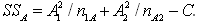 =(0.265322/9) + (0.558142/18) = 0.0000140etc.5. error degree of freedom (dof):dof = 26 – (1+2+2+2+2+2+2+2+2+4) = 5By the error degree of freedom more than 0, F ratio can calculate without “pooling” treatment. The pooling process will delete insignificant factors of experiment until the total of error dof is more than zero. 6. factor of Mean Square variance (MS):
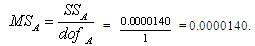 etc.7. factor F ratio:
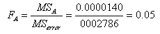 etc.8. factor effect in % (p):
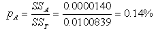 etc.
etc.
References
| [1] | Dobrzanski L.A., Domagala J., Silva J.F., “Application of Taguchi Method in the Optimization off Filament Winding of Thermoplastic Composites”, Archives of Material Science and Engineering, 2005 |
| [2] | D.J. Burr, “Experiments on Neural Net Recognition of Spoken and Written Text”, IEEE Trans. Acoust. Speech Signal Process. 36 (7), (1988) 1162–1168. |
| [3] | Benardos P.G, Vosniakos G.C., “Optimizing Feedforward Artificial Neural Network Architecture”, Elsevier, Engineering Applications of Artificial Intelligence 20 (2007) 365–382. |
| [4] | Jhon F.C. Khaw, B.S. Lim, Lennie E.N.Lim, “Optimal Design of Neural Networks Using the Taguchi Method”, GINTIC Institute of Manufacturing Technology, Nanyang Avenue, Singapura, 1994. |
| [5] | Rajkumar T., Bardina Jorge, “Training Data Requerment for a Neural Network to Predict Aerodynamic Coefficient”, NASA Ames research center, Moffet Field, California, USA. |
| [6] | Yu Huang Chien, Hui Chen Tien, Chung Chen Ching, Ting Chang Ya, Optimizing Design of Back Propagation Networks using Genetic Algorithm Calibrated with the Taguchi Method, SHU-Te University, Taiwan. |
| [7] | Hsu M. William, Evolutionary Computation and Genetic Algorithm, Kansas State Univ., USA, 2006. |
| [8] | Davis Lawrence, “Genetic Algorithms and their Applications”, President of Tica Associates |
| [9] | Phadke S. Madhav, Introduction to Robust Design (Taguchi Approach), Phadke Associates Inc., 2006. |
| [10] | Krottmaier J., Optimizing Engineering Design, McGraw-Hill, England, 1993 |
| [11] | Braspenning P.J., Thuijman F., Weijters A.J.M.M., “Artificial Neural Network”, Springer – Verlag, Berlin, 1995. |
| [12] | Roy Ranjit, A Primer on the Taguchi Method, Van Nostrand Reinhold, USA, 1990. |
| [13] | Fowlkes, W. Y., & Creveling, C. M.,”Engineering methods for robust product design: using Taguchi methods in technology and product development”, MA, 1995. |
| [14] | Field Andy, Discovering Statistic using SPSS, Sage Publication Ltd, London, 2006. |
| [15] | Cohen, J., Statistical power analysis for the behavioural sciences, Hillsdale, New Jersey: Lawrence Erlbaum Associates, 1988. |
| [16] | Montana J. David, Davis L., Training Feedforward Neural Network using Genetic Algorithm, BBN System & Technologies Corp., Cambridge, UK. |
| [17] | Fausett Laurene, Fundamentals of Neural Network, Florida Institute of Technology, Prentice Hall International, Inc, USA, 1994. |
| [18] | Shanthi D., Sahoo G., Saravanan N., “Evolving Connection Weights of Artificial Neural Networks using Genetic Algorithm with Application to the Prediction of Stroke Disease”, International Journal of Soft computing, 2009. |
| [19] | Bolboaca D. Sorana, Jantchi Lorentz, “Design of Experiment: useful Orthogonal Arrays for Number of Experiments from 4 to 6”, Entropy, 2007. |
| [20] | G. Ambrogio and L.Filice, “Application of Neural Network Technique to Predict the Formability in Incremental Forming Process”, University of Calabria, Italy, 2009 |
| [21] | Masters Timothy, Practical Neural Network Recipes in C++”, Academic press INC., 1993. |
 Abstract
 Reference
 Full-Text PDF
 Full-Text HTML