Emran Tohidi
Department of Mathematics, Islamic Azad University, Zahedan Branch, Zahedan, Iran
Correspondence to: Emran Tohidi , Department of Mathematics, Islamic Azad University, Zahedan Branch, Zahedan, Iran.
| Email: |  |
Copyright © 2012 Scientific & Academic Publishing. All Rights Reserved.
Abstract
The purpose of this study is to give a Bernoulli polynomial approximation for thesolution of hyperbolic partial differential equations with three variables and constant coefficients. For this purpose, a Bernoulli matrix approach is introduced. This method is based on taking the truncated Bernoulli expansions of the functions in the partial differential equations. After replacing the approximations of functions in the basic equation, we deal with a linear algebraic equation. Hence, the result matrix equation can be solved and the unknown Bernoulli coefficients can be found approximately. The efficiency of the proposed approach is demonstrated with one example.
Keywords:
Bernoulli Polynomial Solutions, Two-dimensional Linear Hyperbolic Equation With Constant Coefficients, Bernoulli Matrix Method
1. Introduction
When a mathematical model is formulated for a physical problem, it is often represented by partial differential equations, that are not solvable exactly by analytic techniques. Therefore, onemust resort to approximation and numerical methods. For example,theTelegraph equation (as a hyperbolic partial differential equation) is commonly used in signal analysis for transmission and propagation of electrical signals and also has applications in other fields (see[1] and the references therein). We also note that,the differential equationsaresometimes linear in real world as is shown in papers[2, 3].The solution of linear hyperbolic partial differential equations clarifies the linear phenomena which occur in many systems like as biology, engineering, aerospace, industry etc. In the recent years, noticeable progress has been made in the construction of the numerical solutions for linear partial differential equations, which has long been a major concern for both mathematicians and physicists.The various methods for solving linear hyperbolic partial differential equations are introducedin[4].Since the beginning of 1994 several matrix (such as Legendre, Chebyshev, Bessel, Lagurre, Hermite, Bernstein etc.) approachesfor solving linear differential, integral, integro- differential, difference, and integro-difference equations, havebeen presented in many papers by Sezer and Cowork ers[4–11]. In this study, and in the light of the above mentioned methods (and by generalizing the Bernoulli matrix method for one dimensional PDEs[12]) we propose a new matrix approach which is based on Bernoulli truncated series in three dimension for solving two dimensional hyperbolic partial differential equations with constant coefficients in the following form | (1) |
with the initial conditions | (2) |
and the boundary conditions 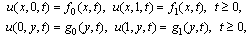 | (3) |
and the solution is approximated by the following Bernoulli truncatedseries 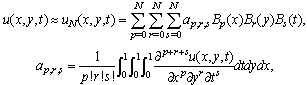 | (4) |
so the Bernoulli coefficients to be determined are  ; where
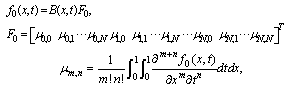
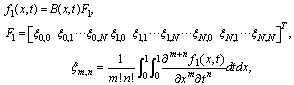
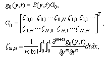
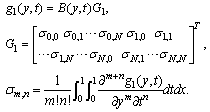
 are known functions
  .The considered partial differential equation (1) arise in connection with various physical and geometrical problems in which the functions involved depend on two or moreindependent variables, on time
  and on one or several space variables[4]. For
  and
and , equation(1) represents a two-space-dimensional damped wave equation (with a source term). The numerical solution of damped wave equations is of great importance in studying wave phenomena.
2. Fundamental Relations
To obtain the numerical solution of the hyperbolic partial differential equation with thepresented method, we first evaluate the Bernoulli coefficients of the unknown function. For convenience, the solution function (4) can be written in the matrix form | (5) |
where is the
  matrix defined as


 and
and where
where On the other hand, the relations between the matrix
  and its derivatives are as follows:
 | (6) |
 | (7) |
 | (8) |
where


 where
where and
and  are
are  and
and  identity matrices respectively.By using the relations (6)-(8)we have
 We can also expand the function
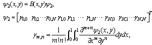
  as a Bernoulli series:
 | (9) |
From (9),one can obtain the following matrix form | (10) |
where with
with .Substituting the expressions (5)–(8) and (10) into equation(1) and simplifying the result, we have the matrix equation
 | (11) |
Briefly, we can write equation(11) in the form | (12) |
where is the
  identity matrix and
  We now present the alternative forms for
  which are important for simplifying matrix forms of the conditions. The simplification in conditions is done only with respect to the variables
 . Therefore we must use different forms for initial and boundary conditions. For the initial conditions (2),
 | (13) |
 while for the boundary conditions (3),
 | (14) |


 and also we use
 | (15) |

 ,
, Notice also that the matrices involved in the right-hand side of Eqs. (2) and (3) are of the form
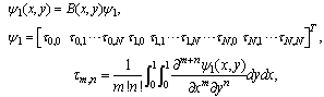 | (16) |
 | (17) |
 | (18) |
 | (19) |
 | (20) |
 | (21) |
By substituting relations (16)–(21) into (2) and (3) and then simplifying the result, we get the matrix forms of the conditions, respectively, as | (22) |
 | (23) |
 | (24) |
 | (25) |
 | (26) |
 | (27) |
 | (28) |
The unknown Bernoulli coefficients are obtained as Where
Where is generated by using the Gauss elimination method and then removing zero rows of the Gauss eliminated matrix. Here
  and
and  are obtained by throwing away the maximum number of row vectors from W and G, so the rank of the system defined in (28) cannot be smaller than
 . This process provides higher accuracy because of the decreasing truncation error.
3. Accuracy of the Solution and Error Analysis
We can easily check the accuracy of the method. Since the truncated Bernoulli series (4) is an approximate solution ofEq. (1), when the function  and its derivatives are substituted in Eq. (1), the resulting equation must be satisfiedapproximately; that is, for

 and
and (
( positive integer). If max
  =
=  (
( positive integer) is prescribed, then the truncation limit
  is increased until the difference
  at each of the points becomes smaller than the prescribed
  .On the other hand, the error, can be estimated by
  and
and  errors, and the root mean square error (RMS). We calculate the RMS error using the following formula :
 where
where and
and  are the exact and approximate solutions of the problem, respectively, and
  is an arbitrary time
  in
in 
4. IllustrativeExample
This section is devoted to a computational result. We applied the method presented in this work and solved one example. We illustrate our work with the following example. The numerical computations were done using MATLAB v7.12.0. Example.Consider the problem .The initial conditions are given by
 By applying the technique described in the preceding section we find the matrix representation of the equation as follows:
 Solving the above linear system yields to
 which is the exact solution.
5. Conclusions
Two-space-dimensional linear hyperbolic equations with constant coefficients are usually difficult to solve analytically. For this purpose, the present method has been proposed for approximate solutions and also analytical solutions. It is observed that the method has a great advantage when the known functions in the equation can be expanded in Bernoulli series. Moreover, this method is applicable for the approximate solution of parabolic and elliptic type partial differential equations in two space dimensions. The method can also be extended to nonlinear partial differential equations, but some modifications are required.
References
| [1] | M. Dehghan, and A. Shokri, A numerical method for solving the hyperbolic telegraph equation, Numer. Methods Partial Diff. Equ. 24 (2008), 1080–1093. |
| [2] | L. Cveticanin, Free vibration of a strong non-linear system described with complex functions, J Sound Vibrat 277 (2005), 815–824. |
| [3] | L. Cveticanin, Approximate solution of a strongly nonlinear complex differential equation, J Sound Vibrat 284 (2005), 503–512. |
| [4] | B. Bülbül and M.SezerTaylor polynomial solution of hyperbolic type partial differential equations with constant coefficients, Int J Comput Math, 88 (2011), 533-544. |
| [5] | M. Sezer, and M. Kaynak, Chebyshev polynomial solutions of linear differential equations, Int J Math EducSciTechnol 27 (1996), 607–618. |
| [6] | A. Akyüz, and M. Sezer, Chebyshev polynomial solutions of systems of high-order linear differential equations with variable coeficients, Appl Math Comput 144 (2003), 237–247. |
| [7] | M. Gulsu, and M. Sezer, The approximate solution of high-order linear difference equation with variable coefficients in terms of Taylor polynomials, Appl Math Com 168 (2005), 76–88. |
| [8] | M. Sezer, and M. Gülsu, A new polynomial approach for solving difference and Fredholmintegro difference equations with mixed argument, Appl Math Comput 171 (2005), 332–344. |
| [9] | A. Karamete, and M. Sezer, A Taylor collocation method for the solution of linear integro-differential equations, Int J Comput Math 79 (2002), 987–1000. |
| [10] | M. Sezer, A. Karamete, and M. Gülsu, Taylor polynomial solutions of systems of linear differential equations with variable coefficients, Int J Comput Math 82 (2005), 755–764. |
| [11] | A. Akyüz and M. Sezer,AChebyshev collocation method for the solution of linear differential equations, Int J Comput Math 72 (1999), 491–507. |
| [12] | E. Tohidi, Numerical Solution of Linear HPDEs Via Bernoulli Operational Matrix of Differentiation and Comparison with Taylor Matrix Method, Accepted in Math. Science.Letter. |
 Abstract
 Reference
 Full-Text PDF
 Full-Text HTML