-
Paper Information
- Next Paper
- Previous Paper
- Paper Submission
-
Journal Information
- About This Journal
- Editorial Board
- Current Issue
- Archive
- Author Guidelines
- Contact Us
American Journal of Computational and Applied Mathematics
p-ISSN: 2165-8935 e-ISSN: 2165-8943
2012; 2(3): 86-93
doi: 10.5923/j.ajcam.20120203.04
State and Unknown Inputs Estimations for Multi-Models Descriptor Systems
 Abstract
 Reference
 Full-Text PDF
 Full-Text HTML
Chokri Mechmeche1, Hamdi Habib1, Mickael Rodrigues2, Naceur BenHadjBraiek1
1Laboratoire d'Etude et Commande Automatique des Processus (LECAP), Ecole Polytechnique de Tunisie
2Laboratoire d'Automatique et de Génie des Procédés (LAGEP), CNRS UMR 5007, Université Lyon 1, France
Correspondence to: Hamdi Habib, Laboratoire d'Etude et Commande Automatique des Processus (LECAP), Ecole Polytechnique de Tunisie.
| Email: |  |
Copyright © 2012 Scientific & Academic Publishing. All Rights Reserved.
In this note, the problem of states and unknown inputs estimation of nonlinear descriptor system is considered. The methodology is based on the use of Proportional Integral and Unknown Input Observers. The considered nonlinear descriptor system is transformed into an equivalent multi-models form by using the Takagi-Sugeno (T-S) approach. In this paper, the design methods of both proportional integral observers and unknown inputs observers for descriptor multi-models are described in detail. Sufficient conditions of stability analysis and gain matrices determination are performed by resolving a set of Linear Matrices Inequalities (LMIs). The design method offers all the degrees of design freedom, which can be utilized to achieve various desired system specifications and performances and, thus, has great potentials in applications. A numerical example is employed to show the design procedure of these two observers and illustrate the effect of the proposed approach.
Keywords: Nonlinear Descriptor System, Multi-Model Descriptor System, Proportional Integral and Unknown Input Observer, LMIs
Article Outline
1. Introduction
- Nonlinear descriptor processes are usually described by analytical models. These models include both dynamic and static relations. Consequently this formalism can model physical constraints or impulsive behavior due to an improper part of the system. Descriptor systems appear in many fields of system design and control such as con- strained robots, power systems, hydraulic or electrical networks. For conventional systems, various approaches have been proposed to design observers. The observer classically used, within the framework of linear systems, is known as Luenberger observer or with profit Proportional[7]. In presence of unknown disturbances affecting system[13], the state estimation provided by this type of observer, is considerably degraded. In order to improve the observer design with respect to the disturbances, an ob- server with Proportional Integral gain can be used. Indeed, this observer makes it possible to integrate certain degree of robustness in state estimation thanks to the integral action[3]. Like to ordinary system theory, the problem of designing observer for descriptor linear system has been considered by many authors. Some approaches are lead to the construction of full-order and reduced-order observers[12]. Othersapproaches develop the concept of singular value decompositions and generalized inverse matrix[10] in order to construct the state vector for this class of systems. Some researchers have also introduced the integral term in observer design for descriptor linear systems. Indeed, in[1] and[2], a design approach of Proportional Integral Observer (PIO) for continuous time descriptor linear systems has been proposed. Koenig et al.[6] have investigated the Luenberger full-order and reduced order PIO with unknown inputs. However, few works have been done to design observers for nonlinear descriptor system except for[5]. In a recent work of Kaprielian et al.[17], a state observer based on the linearization technique of nonlinear descriptor systems with application to a physical process has been developed. The design of these algorithms can become very difficult even impossible according to the type and the complexity of the employed model, from where the importance to have a mathematical model of the system where it’s at the same time, simple and precise. The multi-models approach is a powerful technique of modeling nonlinear systems which make it possible to get a good compromise between the precision and the complexity of the model[14]. Multi-models are recognized for their capacity to take into account the changes in the operating mode of the system and to reproduce its behavior with precision in a broad operating range. Moreover, they offer mathematical properties which can be profitable during the design of observers. More recently, few results have been generalized to the descriptor multi- models. In[4], a state estimation method for singular multi-models with measurable decision variables affected by unknown inputs has been presented. This proposed observer has been applied to fault detection. In[8] and[9] the problem of fault detection isolation and estimation for LPV polytopic descriptor system has been studied by using unknown inputs observer and proportional integral observer. From these works and others, state estimation as well as unknown inputs is very significant in command or diagnosis of systems. This has motivated us to study these problems for descriptor multi-models by both unknown inputs and PI observers. Thus some new results are proposed in this paper, a comparison study between two types of observers is presented. This comparison wants to underline the differences for the design of such observers and also to compare the estimation performances of them. This discussion wants to lead us which of these two observers are less restrictive for nonlinear descriptor systems described by a multi-models approach.This paper is organized as follows: in Section 2 the multi- models structure of nonlinear descriptor systems is introduced. In Section 3, we study the structure and the design of the proposed proportional integral and unknown inputs multi-observer. An illustrative example is considered in section 4.
2. Multi-models Singular System
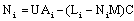
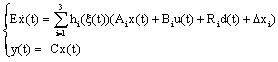
- Consider the following nonlinear descriptor system
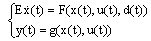 | (1) |
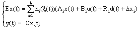 | (2) |
 | (3) |
 | (4) |
 | (5) |
3. Proportional Integral (PI) Muti-Observer Structure
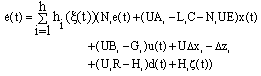
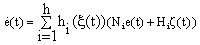
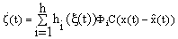
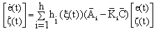
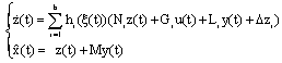
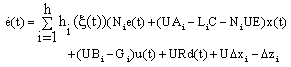
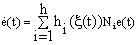
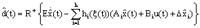
- In the deterministic case, the Proportional Integral Multi- 0bserver (PIMO) is characterized by the use of an integral term of the estimation outputs error[11]. The equations which govern the PIMO are as follows:
 | (6) |
 | (7) |
 | (8) |
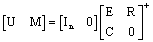
 Let U ∈ Rnxn a real matrix such that:
 | (9) |
 | (10) |
 . Then, for
  the derivative unknown inputs is:
 | (11) |
 | (12) |
 | (13) |
 | (15) |
 | (16) |
 | (17) |
 | (18) |
 | (19) |
 | (20) |
 | (21) |
 | (22) |
3.1. PI Observer Design
- Since rank[ET CT]T, and from (18) we obtain,
 | (23) |
 | (24) |
 | (25) |
 | (26) |
 | (27) |
 | (28) |
 | (29) |
 | (30) |
 | (31) |
 The remaining problem is to find the matricessuch that the state estimation error converges asymptotically to zero.
 3.2. Existence Conditions
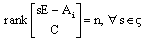
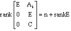
- The PIMO (6) exists if and only if the pair is detectable ∀ i = 1,..., h. The following theorem gives the existence conditions of this PIMO.Theorem 1.[6] The PIMO (6) for the multi-models descriptor system (2) converge asymptotically to zero, if and only if the following conditions are hold:i.
 ii.
ii. 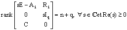 So, it remains to determine the gain
  of the PIMO ensuring the convergence to zeros of the estimation errors. One uses here, the second Lyapunov method.Theorem 2. The PIMO (6) is asymptotically stable, if there exists a common positive definite matrix Q and matrices
  such that:
 | (32) |
 . The stability condition for the dynamic error yields that the time derivative of the Lyapunov function should be negative definite. Using the equation (31), the function
 is derived such as:
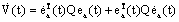
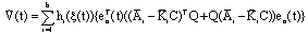 | (33) |
 | (34) |
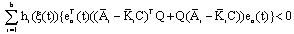
 =1, hi(ξ(t))≥0 and ∀ ea(t)≠0, then (34) is satisfied if:
 For
For , the above inequalities become
 A solution in Q and Wi satisfying LMIs (32) can be found.The observers gains can be deduced as:
  Then, the design of PIMO is achieved and their parameters are given by (28), (29), (15), (16) and (24).To ensure the rate of estimation error convergence, one defines in the left part of the complex plan a bounded area S with a line of abscissa (−α) where α ∈ R+. The LMIs (32) must be replaced by the following LMIs.
 | (35) |
 .
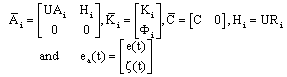
.4. Unknown Input Multi-Observer Structure
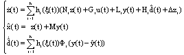
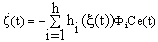
- The Unknown Inputs Multi-Observer (UIMO) design for descriptor multi-models is addressed in this subsection. Two parts are studied, the first is dedicated to the state estimation, in the second, an applicability of the disturbance estimate is considered. So, taking the descriptor model (2) with a constant matrix disturbance i.e. Ri=R, the proposed UIMO has the following form:
 | (36) |
 | (37) |
 | (38) |
 | (39) |
4.1. UIMO Design
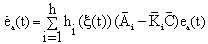
- After checking the convergence conditions (theorem 1), the design of the UIMO (36) consists in finding gains matrices Ki such that the equation (39) is stable. By using (27) and (28), the inequalities (32) can be rewritten as:
 | (40) |
 | (41) |
 | (42) |
 | (43) |
 | (44) |
 | (45) |
 | (46) |
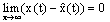
 is a full column rank[12].At this step, the UIMO makes it possible to rebuild the state of the system whatever the presence of the unknown inputs; it is based on the methods of decoupling of the unknown inputs with respect to the estimation error. However, the most critical problem into the design of such UIMO is to solve the equation (38). This decoupling problem is restrictive when the disturbances matrices Ri are different for all the operating point. On the other hand, the PIMO does not decouple the unknown inputs and then its design does not suffer of this problem. The PIMO design is more easy by considering this problem but the restriction for the PIMO is to consider that disturbances have slow variation i.e.
  . By summarizing these observers design, the design method of the PIMO is less restrictive.
4.1. Unknown Inputs Estimation
- Under steady state condition, the state estimation error converges to zero, then substituting the true state x(t) by its estimate
 and the unknown inputs d(t) by its estimated
 in the multi-models (2) and for hypothesis Ri = R, we obtain:
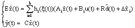 | (47) |
 | (48) |
5. Illustrative Example (A Rolling Disc)
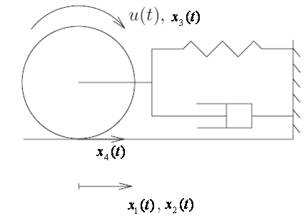
- Consider a singular nonlinear system given by the set of differential and algebraic equations (DAE)[16]. The model describes a disc rolling on surface without slipping figure 1. The disc is connected to a fixed wall with a nonlinear spring and a linear damper. The spring has a positive coefficient k. The damping coefficient of the damper is given by a positive parameter b. The radius of the disc is r, its inertia is given by J and the mass of the disc is m.
 | Figure 1. A rolling disc |
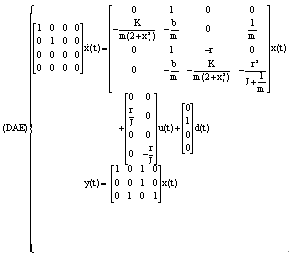 The state vector of this model is given by:x1 ( t): The position of the center of this discx2 ( t): The translational velocity of the same point.x3 ( t): The angular velocity of the disc.x4 ( t): The contact force between the disc and the surface.The control input is denoted u(t) and is a torque applied at the center of the disc.Let us: K = 100 Nm-1, b = 30, m = 40 Kg, r = 40 cm andJ = 0 .5 .m .r2 = 3. 2Kgm-2.
5.1. Multi-models Representation
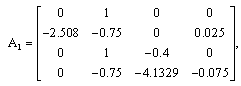
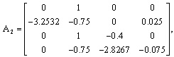
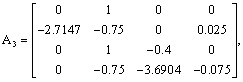
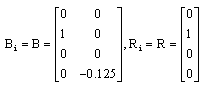
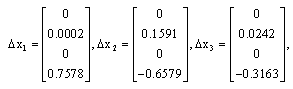
- The nonlinear (DAE) can be approximated by three local models interpolated by convex weighting functions as follows:
 The numerical values of those matrices are as follows:
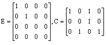
 The weighting functions depend on the measurable state x3(t) as follows:
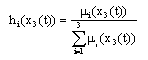 where are defined by:
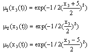 For
For 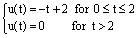 and d(t) an unknown input applied for 5 ≤ t ≤ 10. The simulation of the nonlinear system and the multi-models representation is given by the following figures.
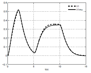 | Figure 2. x1 of nonlinear model and x1 of the multi-models |
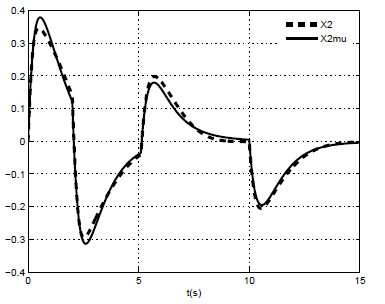 | Figure 3. x2 of nonlinear model and x2 of the multi-models |
 | Figure 4. x3 of nonlinear model and x3 of the multi-models |
 | Figure 5. x4 of nonlinear model and x4 of the multi-models |
5.2. State Estimation
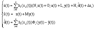
- ● PI multi-observer matrices: The proportional integral multi-observer is represented by:
 The existence of the multi-observer is checked. A solution satisfying the inequality (35) can b e found by using the LMI Toolbox. Then, these inequalities (35) are fulfilled with:
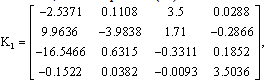
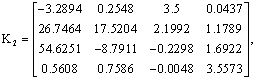
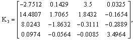
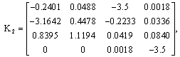
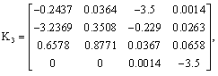
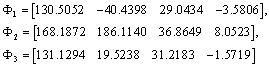 where Ki are the proportional gains matrices and ϕi are the integral gains matrices. The other parameters of the PIMO are given by (14) to (14), (24), (28) and (29).● UIMO matrices: The UIMO (36) is designed by solving the inequalities (40). Then, their obtained gains matrices are:
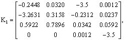
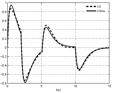
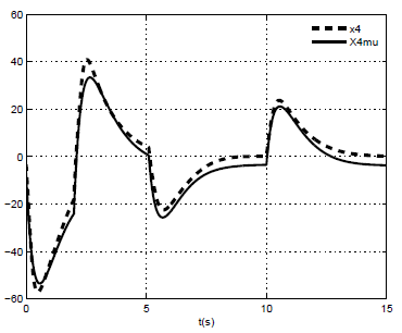
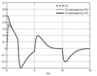
 The other matrices are obtained based on the equations(43) and (46).● Comparison performances between PIMO and UIMO: To evaluate the performances of both PIMO and UIMO in the state and unknown inputs estimation, the following simulation results are given under the same inputs and initial conditions of these observers.The behavior of the PIMO is shown in the figures (6) to (9). It is observed that for both PI and UI multi-observer, the estimated states can closely track the original states. However, the PIMO rebuilds the state by using the estimate of the unknown inputs, contrary to the UIMO which completely decouples the unknown inputs from the state and thus allows a better estimation.
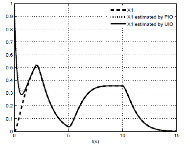 | Figure 6. x1(t) and their estimated by PIMO and UIMO |
 | Figure 7. x2(t) and their estimated by PIMO and UIMO |
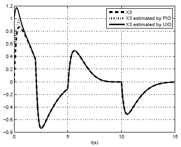 | Figure 8. x3(t) and their estimated by PIMO and UIMO |
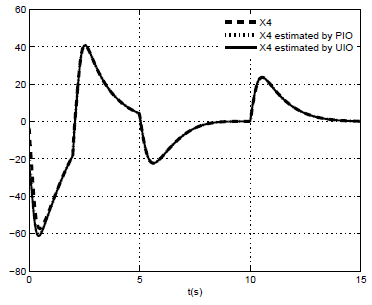 | Figure 9. x4(t) and their estimated by PIMO and UIMO |
5.3. Unknown Inputs Estimation
- Estimated unknown input by booth PIMO and UIMO, is given in the following figure.
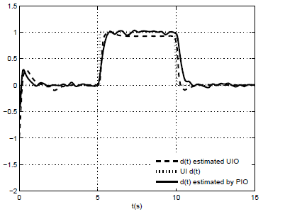 | Figure 10. Unknown input d(t) and their estimated by PIMO and UIMO |
6. Conclusions
- Performances and design comparison of the state and unknown inputs estimation between Proportional Integral and Unknown Inputs Multi-Observers based on a multi- models approach, for nonlinear descriptor system with unknown inputs has been studied. The nonlinear descriptor system is represented by a set of sub-models where each ones is valid in an operating zone. The PIMO provides a good estimation of the state variables but worse unknown inputs estimation than the UIMO. However, the design of UIMO is more restrictive than the PIMO design. The existence conditions for these both multi-observers and an LMI-based computation have been established. The proposed example illustrates the effectiveness of these proposed multi- observers and allows to compare both state and disturbance estimation.