-
Paper Information
- Next Paper
- Paper Submission
-
Journal Information
- About This Journal
- Editorial Board
- Current Issue
- Archive
- Author Guidelines
- Contact Us
American Journal of Computational and Applied Mathematics
p-ISSN: 2165-8935 e-ISSN: 2165-8943
2012; 2(3): 64-72
doi: 10.5923/j.ajcam.20120203.01
Two Different Regimes of Fingerprint Identification – A Comparison
 Abstract
 Reference
 Full-Text PDF
 Full-Text HTML
Terje Kristensen
Departement of Computer Engineering, Bergen University College, Nygårdsgaten 112, N-5020 Bergen, Norway
Correspondence to: Terje Kristensen, Departement of Computer Engineering, Bergen University College, Nygårdsgaten 112, N-5020 Bergen, Norway.
| Email: |  |
Copyright © 2012 Scientific & Academic Publishing. All Rights Reserved.
In this work a hybrid technique for classification of fingerprint identification has been developed to decrease the matching time. For classification, a Support Vector Machine (SVM) and a Multi-Layered Perceptron (MLP) network are described and used. Automatic Fingerprint Identification Systems (AFIS) are widely used today, and it is therefore necessary to find a classification system that is less time-consuming. The fingerprint patterns generated are based on minutiae extraction from a thinned fingerprint image. The given fingerprint database is decomposed into four different subclasses. Two different classification regimes are used to train the systems to do correct classification. The classification rate has been estimated to about 87.0 % and 88.8% of unseen fingerprints for SVM and MLP classification respectively. The classification rate of both systems is only differing marginally.A benchmark test has been done for both systems. The matching time is estimated to decrease with a factor of about 3.7 compared to a brute force approach.
Keywords: Automatic Fingerprint Identification System, Support Vector Machine, Multi-Layered Perceptron, Backpropagation algorithm, Benchmark Test
Article Outline
1. Introduction
- The first Automatic Fingerprint Identification System (AFIS) was developed in 1991, and since then, there has been an enormous progress in the field. Due to the ever-growing capabilities of computers and great achievements in research, the recognition rate has improved significantly. There is nevertheless a huge amount of work still to be done. The current work in this field concentrates on reducing the computation time for feature extraction and matching. Embedded fingerprint systems supporting instant identification or verification are increasingly used, and the computation time for these processes is thus an important research field. One way to decrease this time is to divide the fingerprint database into different subclasses based on specific properties, such that only a part of the fingerprints needs to be considered for matching. The uniqueness of fingerprints has been widely tested, and two identical fingerprints have still not been found (Pankanti et al., 2002). However, current fingerprint identification systems do not use all the discriminating information present in a fingerprint, and the probability of finding two identical fingerprints using the systems therefore increases. A lot of work is being done today to decide whichinformation in fingerprints should be used to keep the uniqueness. In addition to this work, the current work in this field concentrates on reducing the computation time for feature extraction and matching. Various methods have been used for classification. In this paper, both an Artificial Neural Network (ANN) and a Support Vector Machine (SVM) approach have been used for classification. Both networks are given the same feature vector as input, based on Computation of the Poincare index. This method was first proposed by Jain, Prabhakar and Hong in 1999 (Jain et al., 1999). Among all the biometric techniques fingerprint identification is today the most widely used biometric identification form. It has been used in numerous applications. The problem is to develop algorithms which are robust to noise in the fingerprints and are able to deliver accuracy in real time. Different matching techniques can be used for fingerprint identification. In this paper a matching technique based on minutiae extraction from the thinned fingerprint image is used. Such a technique is based on that the ridges of a fingerprint carries certain kind of features. If one considers the ridges as lines, there will be several occurrences in the fingerprint where the line ends or splits into two parts. These features are referred as minutiae.All the minutiae in a fingerprint form a minutiae structure that can be used to distinguish one fingerprint from another. In this paper we are concentrating on bifurcation and ridge endings minutiae. By examining a minutiae structure extracted from the fingerprint one may matched it against structures in other fingerprints.Fingerprint matching algorithms vary greatly in terms of false positive and false negative errors.They may also vary with respect to features such as image rotation invariance and independence from a reference point given as the center or the core of the fingerprint pattern.
2. Background
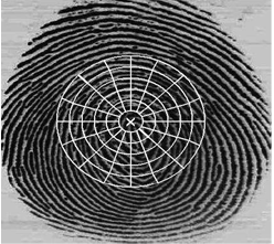
- In an automatic fingerprint identification system (AFIS), the fingerprint databases can be huge, often tens of thousands of fingerprints. If you were supposed to check for similarity between the query fingerprint and every other fingerprint in the database, it can take an enormous amount of time.
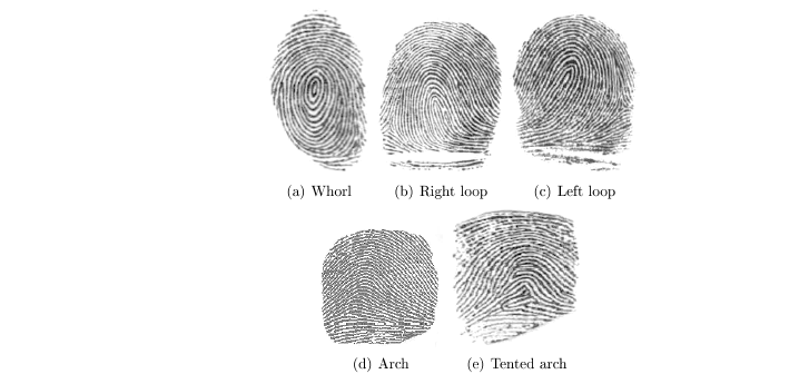 | Figure 1. Five major fingerprint classes |
2.1. Singularities
- Three singularities can be found in a fingerprint to distinguish between the classes. These three singularities are the loop, the delta and the whorl. A whorl fingerprint contains one or more ridges that make a complete 360-degree path around the centre of the fingerprint. Two loops (or one whorl) and two deltas are present. The deltas are placed under the whorl, one at the right and one at the left side. A loop fingerprint has one or more ridges that enter from one side, curves back and exits at the same side as they entered. In a left and right loop, the ridges enter from the left side and the right side, respectively. A loop and a delta singularity are present, with the delta under the loop, at the left in a right loop fingerprint and at the right in a left loop fingerprint. An arch fingerprint has ridges that enter from one side, rises to a small bump and exits at the opposite side. When no singularities are present, this will make the classification of the class rather difficult. A tented arch fingerprint contains one or more ridges that enter from one side, loops in a high curvature and exits at the opposite site. When one loop and one delta singularity are present, the delta is typically placed right under the loop.It is possible to further subdivide each class into more subclasses, but this is hardly of any practical importance. In poor quality fingerprints it is really difficult to even classify it to the five main classes, and further classification would probably increase the rejection rate. In addition, the complexity in the end renders the classification incapable of improving the identification time anymore.
2.2. Different Methods
- Many fingerprint classification methods have been proposed in literature. In general, these methods can be categorised into five approaches (Maltoni, et al., 2005):• rulebased• syntacticbased• structure based • statistical based • neural network based In this work we have concentrated on the statisticalbased and neural network based approach and see how the performance of an AFIS comes out, based on a SVM and an ANN network as classifiers. The current work in this field concentrates on reducing the computation time for feature extraction and matching. Embedded fingerprint systems supporting instant identification or verification are increasingly used, and the computation time for these processes is thus an important research field. One way to decrease this time is to divide the fingerprint database into different subclasses based on specific properties, such that only a part of the fingerprints needs to be considered for matching.
3. Extracting Features
3.1. Extracting Classification Features
- The SVM network needs an input vector to be able to classify the fingerprints. This vector can be made by extracting features of the fingerprint, and then represent these features in a suitable way. We have chosen to create this vector based on a technique proposed by (Maltoni et al., 2005). Here, the authors present a feature vector called FingerCode, which is a vector consisting of 640 feature values. First, a reference point in the fingerprint is be found. We set the core of the fingerprint as the reference point. Then, the image is filtered in eight different directions using different Gabor filters, each enhancing ridges oriented in different angles. Each of these eight images are divided into 80 sectors according to specific rules. The standard deviation of each sector is finally calculated, and these values represent the feature values. The total number of feature values is 640 (8 x 80), and a vector containing these values is used as input vector to both the SVM and the ANN network.
3.2. Reference Point Detection
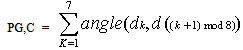
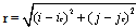
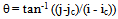
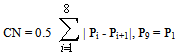
- We have chosen to use the core point as the reference point. This core point is defined as the most northern loop singularity in a fingerprint. A loop singularity can be detected by a method based on the Poincare index proposed in (Jain et al., 1999). Let G be a vector field and C be a curve immersed in G. Then, the Poincare index is defined as the total rotation of the vectors of G along C. Here, G is the vector field associated with an orientation image of the fingerprint. The curve C is a closed path defined as an ordered sequence of the neighbour elements dk of position (i,j) in the orientation image. Then, the Poincare index at position (i,j) is defined as the sum of the orientation differences between adjacent elements of C:
 | (1) |
 | (2) |
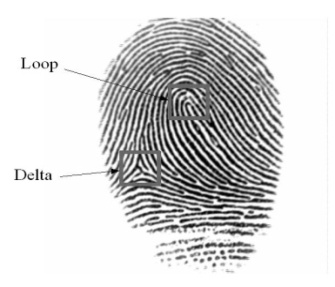 | Figure 2. A loop and a delta singularity in a right loop fingerprint |
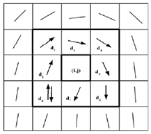 | Figure 3. Computation of the Poincare index in the eight-neighbourhood of pixel (i, j) |
3.3. Gabor Filtering
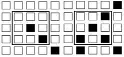
- After the reference point is detected, the image is filtered using eight different Gabor filters. The image needs to be divided into 80 sectors, as illustrated in Figure 4. Here, the reference point is marked with a cross. Note that the innermost band is not divided into sectors, as it contains very few pixels, and the standard deviation will then become very unreliable. Before filtering, each of the 80 sectors has to be normalized, setting the mean and variance to desired values.
 | Figure 4. Computation of the Poincare index in the eight-neighbourhood of pixel (i, j) |
 | (3) |
 | (4) |
 | (5) |
 | (6) |
 | (7) |
3.4. The Feature Vector
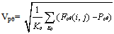
- The feature vector is, as earlier mentioned, a vector consisting of 80 values for each of the eight Gabor filtered images. In each of these images, a section of the fingerprint containing ridges that are parallel to the corresponding filter direction exhibits a higher variation. A section containing ridges that are not parallel to the corresponding filter tends to be smoothed by the filter, which results in a lower variation. The spatial distribution of the variations in the different sectors of the component images can thereby be a good characterisation of the global ridge structure. With this in mind, the feature vector is defined as a vector containing the standard deviation of all 80 sectors in the filtered image for all angles θ (Jain, Farrokhnia, 1999): Let Fpθ(i,j) be the θ-direction filtered image for section Sp. For p ε {0, 1..,79} andθε {0 degrees, 22.5 degrees.., 157.5 degrees}, the feature value is the standard deviation Vpθ, defined as:
 | (8) |
3.5. Scaling
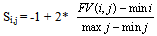
- To improve the classification rate, all feature vectors are scaled before training. The main advantage of scaling is to avoid attributes with big values which dominate those with small values. Another advantage is to avoid numerical difficulties during the calculation. For instance, since the kernel values in Support Vector Machines depend on the inner products of the feature vectors, large attribute values might cause numerical problems. Scaling also makes the training run faster, and decreases the chance of getting stuck in local optima. The feature vectors are linearly scaled to the range [-1,+1]. Each value j in a feature vector i is scaled individually by:
 | (9) |
3.6. Minutiae Extraction
- The ridges of a fingerprint carry certain features. Ridges can end up in ends or splitting of two parts. Such features are referred as minutiae. All the minutiae form a minutiae structure that is used to distinguish one fingerprint from another. To extract minutiae from a fingerprint this can most easily be done by using binarisation technique. Binarisation is the process of converting a gray-scale image into a binary black and white image. The Gabor filtered image is binarised by introducing a threshold value. A thinning process makes the ridges one pixel wide.When the Gabor filtered image is of poor quality some problems may occur which may lead to spurious minutiae. Such minutiae have to be removed from the image. When the fingerprint image is thinned, the minutiae can more easily be extracted from the fingerprint. Only the bifurcation and ridge ending minutiae illustrated in Figure 6 will be handled here.
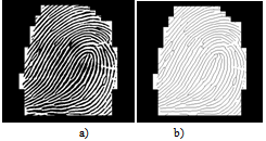 | Figure 5. a) A binarised Gabor filtered image. b) A corresponding thinned image |
 | (10) |
|
 | Figure 6. Examples of ridge an ending point and a bifurcation point |
4. SVM Classification
- Support Vector Machines is a computationally efficient learning technique that is now being widely used in pattern recognition and classification problems (Burges, 1998). This approach has been derived from some of the ideas of the statistical learning theory regarding controlling the generalization abilities of a learning machine (Vapnik, 1999, 1998). In this approach the machine learns an optimum hyper plane that classifies the given pattern. By use of kernel functions, the input feature space may be transformed into a higher dimensional space where the optimum hyper plane can be learnt. By changing the kernel functions many different learning models can be established which makes SVM a very flexible formalism.
4.1. The SVM Classifier
- The basic idea of an SVM classifier is illustrated in Figure 7. This figure shows the simplest case in which the data vectors (marked by 'x's and 'o's) can be separated by a hyper plane. In such a case there may exist many separating hyper planes. Among them, the SVM classifier seeks the separating hyper plane that produces the largest separation margin.
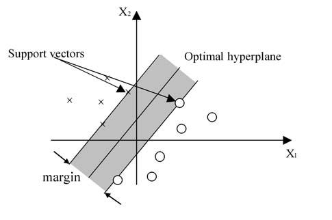 | Figure 7. A Support Vector Machine classification defined by a linear hyper plane that maximizes the separating margins between the classes |
 | (11) |
4.2. SVM Kernel Functions
- The kernel function plays a central role of implicitly mapping the input vectors into a high dimensional feature space, in which linear separability is achieved. The most commonly used kernel functions are the polynomial kernel given by:
 | (12) |
 | (13) |
4.3. SVM Kernel
- The fingerprint database that is used for training and testing for both SVM and MLP network is given in table 2.
|
5. MLP Classification
- A Multi-Layered Perceptron (MLP) network generally contains three or more layers of processing units (Haykin, 2009). Figure 8 shows the topology of a network containing three layers. The bottom layer constitutes the input layer which obtains its input from the environment. The middle layer contains hidden units. The hidden layer has de ability to solve non-linear separable problems.
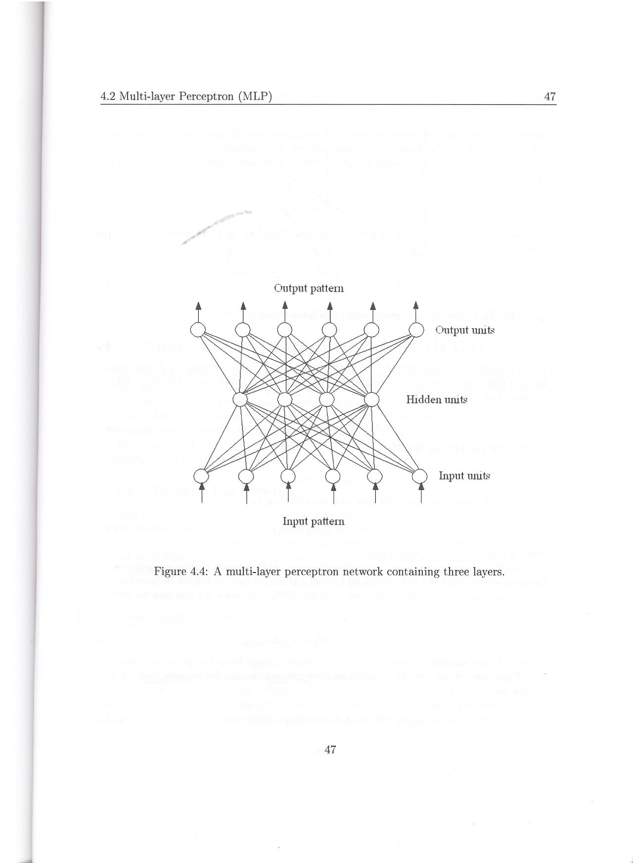 | Figure 8. A MLP network consisting of three layers |
5.1. Training of MLP
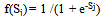
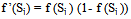
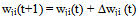
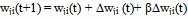
- In the learning phase we present patterns to the network, and the weights are adjusted so that the produced outputs from the output nodes are equal to the target. In fact, we want the network to find a single set of weights that will satisfy all the (input, output) pairs presented to it. Neurons in one layer receive signals from neurons in the layer directly below and send signals to neurons in the layer directly above. Connections between neurons in the same layer are not allowed. Except for the input layer nodes, the network input to each node is the weighted sum of outputs of the nodes in the previous layer. Each node is activated in accordance with the input to the node and the activation of the node. Then, the difference between the calculated output and the target output is calculated. The weights between the output layer, hidden layers and the input layer are adjusted by using this error function. The output of a node is calculated using the sigmoid function f(x) given by:
 | (14) |
 | (15) |
 | (12) |
 | (16) |
 | (17) |
 | (18) |
 | (19) |
 | (20) |
 | (21) |
6. Experiments and Results
6.1. SVM Experiments
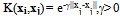
- The SVM is trained using a Radial Basis Function kernel K(xi,xj), given by equation 13.
 | (22) |
|
6.2. MLP Experiments
- The MLP network was also trained by a database according to the numbers specified in table 1. The implementation of the MLP network is based on a network containing 50 hidden nodes. To classify the output from the network we used 4 output units, one for each classification. If a feature vector is classified as a left loop, the correct output is set to the vector {1, 0, 0, 0} and a right loop to {0, 1, 0, 0}. When deciding the parameters of the MLP network, we need to take into consideration the classification performance of unseen patterns, not only the training patterns.Overtraining of an MLP network may be a problem, and the number of iterations and learning rate should be adjusted so that such a situation does not occur. We found that the best results were achieved by setting the learning rate to 0.1 and the momentum to 0.9.Table 4 below shows the classification rate on the testing cases of the MLP network of the different fingerprint classes.
|
6.3. Benchmarking
- A benchmark test was carried out on the total set of fingerprints to measure the average matching time of a fingerprint identification using different subclasses. Matching of two fingerprints (scaling, rotation, translation) takes about 0.268 seconds using the implementation environment defined above. The fingerprint database consisted of 343 fingerprints which mean a total matching time against the entire database of 1 minute and 32 seconds without classification. Using a classification stage against the entire database the average matching time becomes 23 seconds. This time may vary as a tented arch fingerprint takes, for instance, less time since the database contains a smaller amount of fingerprints belonging to this class. The classification time of a fingerprint is less than two seconds. Using a classification stage the matching thereby decrease the matching time by a factor of 92/(23+2) = 3.7.
7. Discussion
7.1. Classification by SVM
- From table 3 we see that SVM failed to classify most of the tented arch fingerprints. However, this may be a result of too few training instances belonging to the tented arch class. SVM also performed better classification of left loops and right loops compared to the classification of whorls. This may be caused by the limited region-of-interest used to calculate the feature vector, causing many whorls to be wrongly classified as loops. There are two main classes of whorls, classic whorl and double loop. The double loop causes often a classification problem. This is because the region-of-interest centered in the core looks quite similar in double loops and normal loops. Thereby, they can easily be misclassified as loops. A solution could be to increase the region-of-interest, but this would also increase the rejection rate, as more sectors would be outside the fingerprint area or even outside the entire image.The experiments have shown that a SVM network is able to do a correct classification with a rate of 87.0% on a four-class classification problem. In (Karu, Jain, 1996), a classification algorithm based on the number of cores and deltas, and their relative positions, is presented. The authors achieved a correct classification rate of 85.4% on a five-class classification task. In (Cappelli, Lumini, Maio, Maltoni, 1999) one has partitioned the directional image into connected regions according to their fingerprint topology, thus giving a synthetic representation which can be exploited as basis for classification. This method achieved a correct classification rate of 92.1% on a four-class classification task. We see that our SVM classifier is not able to match these results at the moment.However, training with a larger fingerprint database than we had available would probably also increase the performance rate of our classification, as the SVM network then is capable to better distinguish important differences between the fingerprint classes.
7.2. Classification by MLP
- From table 4 we can notice that MLP failed in classifying most of the tented arch fingerprints, but again this may be a result of too few training instances belonging to the tented arch class. The MLP network also performed better in classification of left loops and right loops than classification of whorls, the same results as we obtained for SVM. And again this may be caused by the limited region-of-interest used to calculate the feature vector, causing many whorls to be wrongly classified as loops such as in the SVM case. The experiments show us that a MLP network is able to classify correct with a classification rate of 88.8 % on a four-class classification problem. This is a slightly better result than obtained by using SVM as a classifier. However, compared to results obtained in (Jain, Prabhakar, Hong, 1999) this is not so impressive. The authors have used an approach similar to the one used in this paper, with the FingerCode as feature vector and an equivalent feed-forward Multi-Layer Perceptron (MLP) network as the classifier. By using a MLP network one was able to achieve a correct classification rate of 86.4% on a five-class classification task and 92.1% on a four-class classification task. But, again the difference in performance between our approach and the approach used by these authors may be a result of that the training database is too small. Another aspect is that our system is based on a matching process of fingerprint identification based on minutia matching where the minutiae have been extracted from the thinned image of a fingerprint. The two approaches are therefore not quite comparable.
8. Conclusions
- To decrease the identification time of an AFIS, it is necessary to classify the fingerprints into different subclasses, such that a query fingerprint does not have to be tested against every fingerprint in the database. To solve this problem, we have implemented a classification stage in the AFIS by using either a SVM or a MLP network as a classifier. A MLP classifier is able to classify different unseen fingerprints with a performance rate of approximately 89.0%. In addition, by introducing such a classification stage one is also able to reduce the average matching time of a fingerprint with a factor of about 3.7. The main objection by the method used so far is that the number of training samples is too small compared to the number of features in the FingerCode vector. We believe that this is the main reason why we have not achieved so good results compared tothe results in the literature. However, by training the MLP with an extended training database we believe that the total performance rate will improve, and be comparable or better to the results achieved in the literature. Compared to SVM a MLP network is able to do a slightly better classification (Kristensen, 2010). However, we also know that a SVM classifier becomes better when the dimension of the input space becomes higher. It is therefore difficult to predict which type of network is going to be used as the final classifier in a future developed AFIS.