GBSL. Soujanya 1, Y. N. Reddy 1, K. Phaneendra 2
1Department Mathematics, National Institute of Technology, Warangal, 506004, India
2Department Mathematics, Kakatiya Institute of Technology and Science, Warangal, 506015, India
Correspondence to: K. Phaneendra , Department Mathematics, Kakatiya Institute of Technology and Science, Warangal, 506015, India.
| Email: |  |
Copyright © 2012 Scientific & Academic Publishing. All Rights Reserved.
Abstract
In this paper, an exponential fitted method is presented for solving singularly perturbed two-point boundary value problems with the boundary layer at one end (left or right) point via deviating argument. The original second order boundary value problem is transformed to first order differential equation with a small deviating argument. This problem is solved efficiently by using exponential fitting and discrete invariant imbedding method. Maximum absolute errors of several standard examples are presented to support the method.
Keywords:
Singular Perturbation Problems, Boundary Layer, Deviating Argument, Linear Approximation, Maximum Absolute Errors
1. Introduction
Numerical solution of boundary value problems in singularly perturbed second-order, generally nonlinear, ordinary differential equations, is an established research area. Many numerical methods have been proposed for the solution of singularly perturbed two point boundary value problems. It is well known that the standard centered difference scheme has order O(h2), but it gives a non-physical oscillation in the numerical solution when applied on a coarse mesh because of a boundary layer. In order to remove this non-physical oscillation phenomena, it is necessary to use sufficiently small step size h compared to , theoretically. But it is not practical to use finer mesh than
  in real application when ε is very small. Adaptive methods present one possible approach. The adaptive methods strive to automatically concentrate computational grids within boundary layers, interior layers, or other kinds of local solution structures typical of the singularly perturbed ODE’s.For the analysis of this type of problems the readers can refer to the books by Bender and Orszag[1], O’Malley[8], Nayfeh [7], Doolan[3] and Roos[14].Brian J. McCartin[2] presented exponential fitted schemes for the numerical approximation of delayed recruitment/ renewal equations. Fevi Erdogan[4] presented an exponentially fitted difference scheme for singularly perturbed initial value problem for linear first-order delay differential equation. Mohan K. Kadalbajoo, Vikas Gupta[5] presented a brief survey on numerical methods for solving singularly perturbed problems. Natesan and Bawa[6] constructed a hybrid numerical scheme on a piece-wise uniform Shishkin mesh consisting of cubic spline scheme in the boundary layer regions and the classical finite difference scheme in the regular regions, for solving singular perturbation problems. J.I. Ramos[9] presented exponentially-fitted methods on layer-adapted meshes based on the freezing of the coefficients of the differential equation and integration of the resulting equations subject to continuity and smoothness conditions at nodes. Rao and Kumar[10] presented an exponential B-spline collocation method for self-adjoint singularly perturbed boundary value problem and the method is shown to have second order uniform convergence. Rashidinia et al.[11] used spline in compression to develop the numerical methods for singularly perturbed two-point boundary-value problem. They discussed the convergence analysis of the method and show that proposed methods are second-order and fourth order accurate and applicable to problems both in singular and non-singular cases. Reddy [12] has discussed the numerical solution of singular perturbation problems via deviating arguments. Reddy and Chakravarthy[13] constructed an exponentially fitted finite difference method for solving singularly perturbed two-point boundary value problem. A fitting factor is introduced in a tridiagonal finite difference scheme and is obtained from the theory of singular perturbations. In this paper, we present an exponential fitted method for solving singularly perturbed two-point boundary value problems with the boundary layer at one end (left or right) point via deviating argument. The original second order boundary value problem is transformed to first order differential equation with a small deviating argument. This problem is solved efficiently by using exponential fitting and discrete invariant imbedding method. Numerical results and maximum absolute errors of several standard examples are presented to support the method.
2. Numerical Method
2.1. Left-end Boundary Layer
Consider singularly perturbed linear two-point boundary value problems of the form  | (1) |
with boundary conditions  (2a) and
  (2b)where
  , b(x), f(x) are bounded continuous functions in (0, 1), f(x) > 0 and
  are finite constants. Further, we assume that
  throughout the interval [0, 1], where M is positive constant. This assumption merely implies that the boundary layer will be in the neighbourhood of x = 0.By using Taylor series expansion about the deviating argument
  in the neighbourhood of the point x, we have
 | (3) |
and consequently, equation (1) is replaced by the following first order differential equation with a small deviating argument: | (4) |
where The transition from equation (1) to equation (4) is admitted, because of the condition that
  is small. Now we divide the interval [0, 1] into N equal subintervals of mesh size h=1/N so that
  0, 1, 2,…, N. Here, for consolidations our ideas of the method, we assume that a(x), b(x) and f(x) are constants. Hence, p(x), q(x) and r(x) are constant. Rearranging equation (4) as
  We then apply an integrating factor
  , producing (as in[2])
 Next, integrating from
  , we obtain
 By making use of linear approximation on
  , which we insert into the above equation we have

 | (5) |
After evaluating the integrals in equation (5), we get 
 Let
Let ,
,  Then, we have
 | (6) |
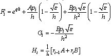
The equation (6) can be written as a tridiagonal system of equations given by | (7) |
where
2.2. Right-end Boundary Layer
We assume that  throughout the interval[0, 1], where M is negative constant. This assumption merely implies that the boundary layer will be in the neighbourhood of x = 1.By using Taylor series expansion about the deviating argument in the neighbourhood of the point x, we have
 | (8) |
and consequently, equation (1) is replaced by the following first order differential equation with a small deviation argument: | (9) |
for  where
where The transition from equation (1) to equation (9) is admitted, because of the condition that
  is small. This replacement is significant from the computational point of view. Now we divide the interval [0, 1] into N equal subintervals of mesh size h=1/N so that
  0, 1, 2,…, N. Here, for consolidations our ideas of the method we assume that a(x), b(x) and f(x) are constants. Hence, p(x), q(x) and r(x) are constant. We then apply an integrating factor
  , producing (as in[2])
 Integrating from
  , we obtain
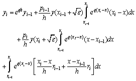 (10)After evaluating the integrals in equation (10), we get
 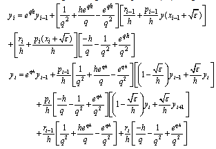 Let
Let  ,
,  Then, we have
 | (11) |
The equation (11) can be written as a tridiagonal system of equations given by | (12) |
where 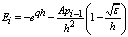
 The tridiagonal system of equations (7) and (12) holds for i=1, 2,…,N-1, we have N-1 linear equations in the N-1 unknowns
  . We assume the matrix of this set of linear equations as
 .Lemma: for all
  and all h=1/N the matrix
  is an irreducible and diagonally dominant matrix.Proof. Clearly,
  is a tridiagonal matrix. Hence,
  is irreducible if its codiagonals contain non-zero elements only. It is easily seen that the codiagonals
  do not vanish for all
  ,
,  and . Hence
  is irreducible.Since
  do not vanish for all
  ,
,  and
and  these expressions are of constant sign. Then obviously,
  Now in each row of
  , the sum of the two off-diagonal elements less than or equal to the modulus of the diagonal element. This proves the diagonal dominant of
  .Under these conditions the discrete invariant imbedding algorithm is stable[10].
3. Numerical Examples
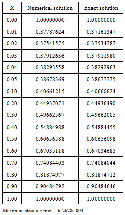
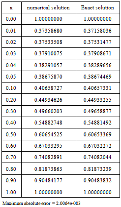
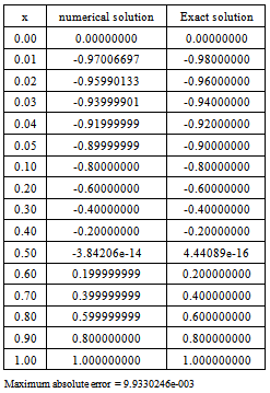
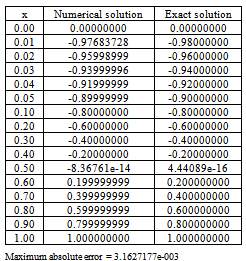
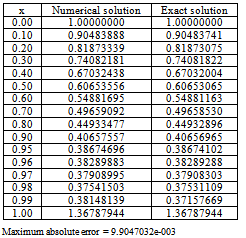
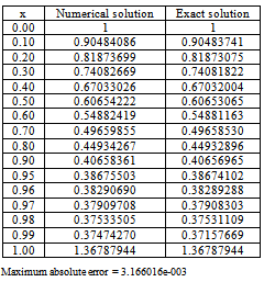
To demonstrate the applicability of the method, we have applied it to three linear singular perturbation problems with left-end boundary layer and two linear problems with right-end boundary layer. These examples have been chosen because they have been widely discussed in literature and because exact solutions are available for comparison. We have also present the maximum absolute errors for the problems. Example 1. Consider the following homogeneous singular perturbation problem ; x∈[0, 1]with y(0) =1 and y(1) =1.The exact solution is given by where
 and
and  The numerical results are given in tables 1 and 2 for different values of
  .
.Table 1. Numerical results of Example1 with

 |
| |
|
Table 2. Numerical results of Example 1 with

 |
| |
|
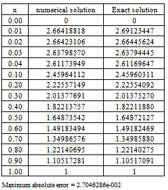
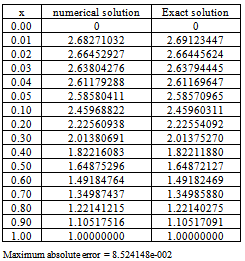
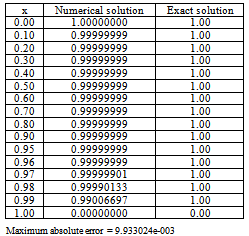
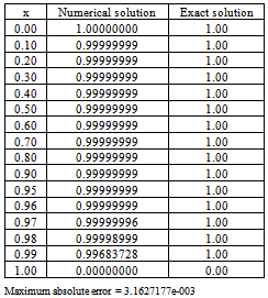
Example 2. Now consider the following non- homogeneous singular perturbation problem  ; x∈[0,1]with y(0) = 0 and y(1) = 1.Clearly this problem has a boundary layer at x = 0.The exact solution is given by
  The numerical results are presented in tables 3 and 4 for different values of
  .
.Table 3. Numerical results of Example 2 with

 |
| |
|
Table 4. Numerical results of Example 2 with

 |
| |
|
Example 3. Consider the following singular perturbation problem  ; x ∈[0,1]with y(0) = 0 and y(1) = 1.The exact solution is given by
  .The numerical results are presented in tables 5 and 6 for different values of
  .Example 4. Consider the following singular perturbation problem
  ; x ∈[0, 1]with y (0) =1 and y (1) =0.Clearly, this problem has a boundary layer at x = 1 i.e., at the right end of the underlying interval.
Table 5. Numerical results of Example 3 with

 |
| |
|
Table 6. Numerical results of Example 3 with

 |
| |
|
The exact solution is given by  The numerical results are presented in tables 7 and 8 for different values of .
Table 7. Numerical results of Example 4 with

 |
| |
|
Table 8. Numerical results of Example 4 with

 |
| |
|
Example 5. : Now we consider the following singular perturbation problem ; x∈[0, 1]with y(0) = 1+exp(-(1+ε)/ε); and y(1) = 1+1/e.
Table 9. Numerical results of Example 5 with

 |
| |
|
Table 10. Numerical results of Example 5 with

 |
| |
|
Clearly this problem has a boundary layer at x = 1. The exact solution is given byThe numerical results are presented in tables 9 and 10 for different values of ε.
4. Discussions and Conclusions
We have presented a numerical method for solving singularly perturbed two-point boundary value problems with the boundary layer at one end (left or right) point via deviating argument and an exponential fitted method. The original second order boundary value problem is transformed to first order differential equation with a small deviating argument. We obtained the tridiagonal system by using exponential fitting and linear approximation and discrete invariant imbedding method is used to solve the system. The method is very easy to implement. Numerical results and maximum absolute errors of standard examples chosen from the literature are presented to support the method.
References
| [1] | Bender, C.M. and Orszag, S.A., Advanced Mathematical Methods for Scientists and Engineers, McGraw-Hill, New York, 1978. |
| [2] | Brian J. McCartin, "Exponential fitting of the delayed re-cruitment/renewal equation", Journal of Computational and Applied Mathematics, vol.136, 343-356, 2001. |
| [3] | Doolan, E.P., Miller, J.J.H. and Schilders, W.H.A., Uniform Numerical Methods for problems with Initial and Boundary Layers, Boole Press, Dublin, 1980. |
| [4] | Fevzi Erdogan, An Exponentially-fitted method for singularly perturbed delay differential equations, Advances in Difference Equations, volume 2009, Article ID 781579, 9 pages, 2009. |
| [5] | Kadalbajoo, M. K., Vikas Gupta., "A brief survey on numerical methods for solving singularly perturbed problems", Applied Mathematics and Computation, vol.217, 3641-3716, 2010. |
| [6] | Natesan, S. and Bawa, R.K., "Second-order numerical scheme for singularly perturbed reaction–diffusion robin problems", JNAIAM J. Numer. Anal. Ind. Appl. Math. vol.2, 177–192, 2007. |
| [7] | Nayfeh, A.H., Problems in Perturbation, Wiley, New York,1985. |
| [8] | O’Malley, R.E., Introduction to Singular Perturbations,Academic Press, New York, 1974. |
| [9] | Ramos, J.I., Exponentially-fitted methods on layer-adapted meshes, Applied Mathematics and Computation, vol. 167,1311-1330, 2005. |
| [10] | Rao, S.C.S. and Kumar, M., "Exponential b-spline collocation method for self-adjoint singularly perturbed boundary value problems", Appl. Numer. Math. vol. 58, 1572–1581, 2008. |
| [11] | Rashidinia, J, Ghasemi, M, and Mahmoodi, Z, "Spline approach to the solution of a singularly-perturbed boun-dary-value problems", Appl. Math. Comput. vol. 189, 72–78, 2007. |
| [12] | Reddy, Y.N., Numerical Treatment of Singularly Perturbed two point boundary value problems, Ph.D. Thesis, IIT, Kanpur, India, 1986. |
| [13] | Reddy, Y.N. and Pramod Chakravarthy, P., "An exponen-tially fitted finite difference method for singular perturbation problems", Appl. Math. Comput. vol. 154, 83–101, 2004. |
| [14] | Roos, G., Stynes, M and Tobiska, L., Numerical methods for singularly perturbed differential equations, Springer Verlag, Berlin, 1996. |
 Abstract
 Reference
 Full-Text PDF
 Full-Text HTML