-
Paper Information
- Next Paper
- Previous Paper
- Paper Submission
-
Journal Information
- About This Journal
- Editorial Board
- Current Issue
- Archive
- Author Guidelines
- Contact Us
American Journal of Computational and Applied Mathematics
p-ISSN: 2165-8935 e-ISSN: 2165-8943
2012; 2(2): 33-41
doi: 10.5923/j.ajcam.20120202.07
MHD-Conjugate Heat Transfer Analysis for Transient Free Convective Flow Past a Vertical Slender Hollow Cylinder
 Abstract
 Reference
 Full-Text PDF
 Full-Text HTML
H. P. Rani , G Janardhana Reddy
Department of Mathematics, National Institute of Technology, Warangal, 506004, India
Correspondence to: H. P. Rani , Department of Mathematics, National Institute of Technology, Warangal, 506004, India.
| Email: |  |
Copyright © 2012 Scientific & Academic Publishing. All Rights Reserved.
In this paper the effects of magnetic field and conduction on the transient free convective boundary layer flow over a vertical slender hollow circular cylinder with the inner surface at a constant temperature are investigated. The transformed dimensionless governing equations for the flow and conjugate heat transfer are solved by using the implicit finite difference scheme. For the validation of the current numerical method heat transfer results for a Newtonian fluid case where the magnetic effect and conduction is zero are compared with those available in the existing literature, and an excellent agreement is obtained. Numerical results for the transient flow variables, average wall shear stress and average heat transfer rate are shown graphically. In all these profiles it is observed that the times needed to reach the steady-state and the temporal maximum increases as the magnetic parameter or conjugate heat transfer parameter increases.
Keywords: Conjugate Heat Transfer, Magneto Hydrodynamic, Natural Convection, Vertical Slender Hollow Cylinder, Finite Difference Method
Article Outline
1. Introduction
- Unsteady natural convection flows over vertical bodies have a wide range of applications in engineering and technology. In manufacturing processes such as hot extrusion, metal forming and crystal growing, heat transfer effects plays an important role. Free convection flow of air bathing a vertical cylinder with a prescribed surface temperature was first presented by Sparrow and Gregg[1] by applying the similarity method and power series expansion. Velusamy and Garg[2] presented the numerical solution for transient natural convection over heat generating vertical cylinders of various thermal capacities and radii. While Fujii and Uehara[3] analyzed the local heat transfer results for arbitrary Prandtl numbers. Lee et al.[4] investigated the similar problem along slender vertical cylinders and needles for the power-law variation in the wall temperature. In general, Ganesan and Rani[5] have investigated the unsteady natural convection flow over a vertical cylinder with variable heat and mass transfer using the finite difference method. Recently, Rani and Kim[6] investigated the unsteady effects for the similar problem with temperature dependent viscosity.In these studies the wall conduction resistance for the convective heat transfer between a solid wall and a fluid flow was neglected considering a thin vertical wall. However, in practical systems the wall conduction resistances have a significant effect in the fluid flow and in the heat transfer characteristics in the vicinity of the wall. Thus the conduction in the solid wall and the convection in the fluid, known as conjugate heat transfer (CHT), should be determined simultaneously. These type of problems are usually referred to as conjugate heat transfer problems, and they have many practical applications, particularly those related to energy conservation in buildings, cold storage installations and cryogenic applications, such as medical and space technology. The CHT problems have been studied by several research groups[7-9] with the help of mathematical models for simple heat exchanger geometries. Gdalevich et al.[10] and Miyamoto et al.[11] reviewed the early theoretical and experimental works of the CHT problems for a viscous fluid. Miyamoto observed that a mixed-problem study of the natural convection has to be performed for an accurate analysis of the thermofluid-dynamic (TFD) field if the convective heat transfer depends strongly on the thermal boundary conditions. Pozzi et al.[12] investigated the entire TFD field resulting from the coupling of natural convection along and conduction inside a heated flat plate by means of two expansions, regular series and asymptotic expansions. Moreover, Vynnycky et al.[13] studied the two dimensional conjugate free convection for a vertical plate of finite extent adjacent to a semi-infinite porous medium using finite difference techniques. Recently, Kaya[14] studied the effects of buoyancy and CHT on non-Darcy mixed convection about a vertical slender hollow cylinder embedded in a porous medium with high porosity.Also, magnetohydrodynamic (MHD) flow and heat transfer processes occur in many industrial applications such as the geothermal system, aerodynamic processes, chemical catalytic reactors and processes, spreading of chemical pollutants in plants. Moreover, effects of thermophoresis on hydromagnetic flow along a flat plate were studied by Chamkha and Camille [15]. Recently, Mamun et al.[16] investigated the effects of magnetic field, viscous dissipation and heat generation on natural convection flow along and conduction inside a vertical flat plate.From the above studies, it can be noted that the CHT on the unsteady natural convective hydromagnetic flow of a viscous incompressible fluid over a vertical cylinder has received very scant attention in the literature. Hence, in the present investigation our attention is focused on the effect of magnetic field on the coupling of conduction inside and the laminar natural convection flow over the outside surface of a vertical slender hollow cylinder. The temperature of the inner surface of the cylinder is kept at a constant value which is higher than the ambient fluid temperature and the temperature of the outer surface is determined by the conjugate solution of the steady-state energy equation of the solid and the boundary layer equations of the fluid flow. The governing equations are solved numerically by the implicit finite difference method to obtain the transient velocity and temperature profiles, coefficient of skin-friction and heat transfer rate for different values of conjugate heat transfer and magnetic parameters.In section 2, a detailed description about the formulation of the problem is given. Also, the governing equations, such as mass, momentum and energy equations of an incompressible fluid flow past a vertical cylinder are derived and non-dimensionalized. In section 3, the details about the grid generation and numerical methods for solving the above governing equations are given. In section 4, transient two-dimensional velocity and temperature profiles, average skin-friction coefficient and heat transfer rate are analyzed. Finally, the concluding remarks are made in section 5.
2. Formulation of the Problem
- An unsteady two-dimensional laminar free convective hydromagnetic flow of a viscous incompressible fluid past a vertical slender hollow cylinder of length l and outer radius
 is considered as shown in Fig. 1. The x-axis is measured vertically upward along the axis of the cylinder. The origin of x is taken to be at the leading edge of the cylinder, where the boundary layer thickness is zero. The radial coordinate, r, is measured perpendicular to the axis of the cylinder. The surrounding stationary fluid temperature is assumed to be of ambient temperature (
 ). The temperature of the inside surface of the cylinder is maintained at a constant temperature of
  , where
  . Initially, i.e., at time
  it is assumed that the outer surface of the cylinder and the fluid are of the same temperature
  . As time increases (
 ), the temperature of the outer surface of the cylinder is raised to the solid-fluid interface temperature
  and maintained at the same level for all time
  . This temperature
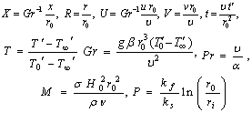
  is determined by the conjugate solution of the steady-state energy equation of the solid and the boundary layer equations of the fluid flow and is discussed elsewhere. It is assumed that the effect of viscous dissipation is negligible in the energy equation. It is further assumed that the interaction of the induced axial magnetic field with the flow is considered to be negligible compared to the interaction of the applied magnetic field
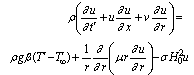
  , with the flow. Under these assumptions, the boundary layer equations of mass, momentum and energy with Boussinesq's approximation are as follows:
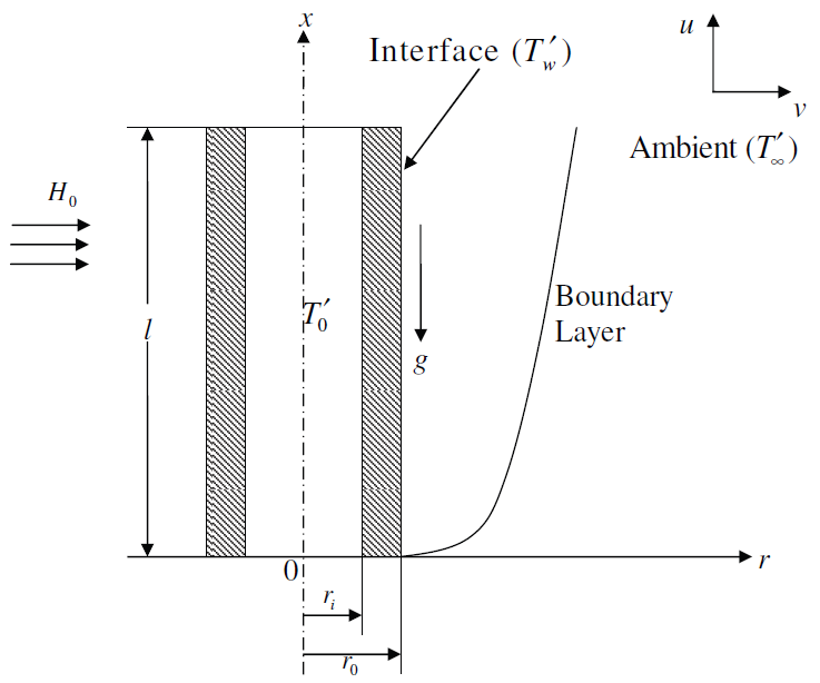 | Figure 1. Schematic of the investigated problem |
 | (1) |
 | (2) |
 | (3) |
 | (4) |
 is the unknown solid-fluid interface temperature and is determined as follows:To predict the outer surface temperature of the cylinder
  , an additional governing equation is required for the slender hollow cylinder based on the simplification that the wall of cylinder steady transfers its heat to the surrounding fluid. Since the outer radius of the hollow cylinder,
  , is small compared to its length, l, the axial conduction term in the heat conduction equation of the cylinder can be omitted. The governing equation for the temperature distribution within the slender hollow circular cylinder is given by Chang[17] as follows:
 | (5) |
 | (6) |
 | (7) |
 | (8) |
 at the interface is given by
 | (9) |
 | (10) |
 | (11) |
 | (12) |
 | (13) |
 | (14) |
3. Numerical Procedure
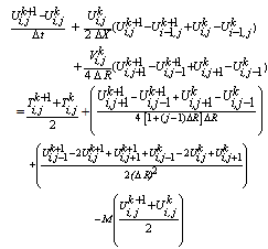
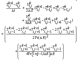
- In order to solve the unsteady coupled non-linear governing Eqs. (11)-(13) an implicit finite difference scheme of Crank-Nicolson type has been employed. The finite difference equations corresponding to Eqs. (11) - (13) are as follows:
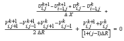 | (15) |
 | (16) |
 | (17) |
 which lies very far from the momentum and energy boundary layers. In the above Eqs. (15)-(17) the subscripts i and j designate the grid points along the X and R coordinates, respectively, where X = i ∆X and R = 1 + (j -1) ∆R and the superscript k designates a value of the time t (= k ∆t), with ∆X, ∆R and ∆t the mesh size in the X, R and t axes, respectively. In order to obtain an economical and reliable grid system for the computations, a grid independent test has been performed. The steady-state velocity and temperature values obtained with the grid system of 100 × 500 differ in the second decimal place from those with the grid system of 50 × 250, and in the fifth decimal place from those with the grid system of 200 × 1000. Hence, the grid system of 100 × 500 has been selected for all subsequent analyses, with mesh size in X and R direction are taken as 0.01 and 0.03, respectively. Also, the time step size dependency has been carried out, from which 0.01 yielded a reliable result.From the initial conditions given in Eq. (14), the values of velocity U, V and temperature T are known at time t = 0, then the values of T, U and V at the next time step can be calculated. Generally, when the above variables are known at t = k ∆t, the variables at t = (k + 1) ∆t are calculated as follows. The finite difference Eqs. (16) and (17) at every internal nodal point on a particular i-level constitute a tridiagonal system of equations. Such a system of equations is solved by the Thomas algorithm [18]. At first, the temperature T is calculated from Eq. (17) at every j nodal point on a particular i-level at the (k + 1)th time step. By making use of these known values of T, the velocity U at the (k+1)th time step is calculated from Eq. (16) in a similar manner. Thus, the values of T and U are known at a particular i-level. Then the velocity V is calculated from Eq. (15) explicitly. This process is repeated for the consecutive i-levels; thus the values of T, U and V are known at all grid points in the rectangular region at the (k + 1)th time step. This iterative procedure is repeated for many time steps until the steady-state solution is reached. The steady-state solution is assumed to have been reached when the absolute difference between the values of velocity as well as temperature at two consecutive time steps is less than
  at all grid points. The truncation error in the employed finite difference approximation is
  and tends to zero as ∆X, ∆R and ∆t → 0. Hence the system is compatible. Also, this finite difference scheme is unconditionally stable and therefore, stability and compatibility ensure convergence.
4. Results and Discussion
- For the validation purpose, the present simulated velocity and temperature profiles are compared with those of the available steady-state, isothermal results of Lee et al.[4] for air (Pr = 0.7) without conduction and magnetic effects i.e., P = 0.0 and M = 0.0, as there are no experimental or analytical studies available to compare with the present problem. The current results are found to be in good agreement with the previous results available in literature as shown in Fig. 2.
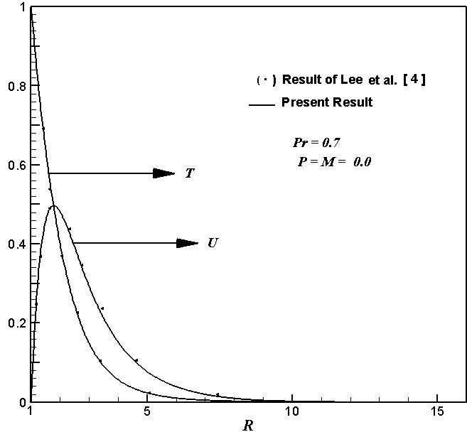 | Figure 2. Comparison of the velocity and temperature profiles |
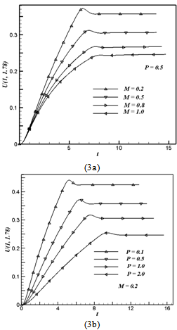 | Figure 3. The simulated transient velocity at (1, 1.78) for (a) variation of M ; (b) variation of P |
4.1. Velocity
- The simulated transient velocity (U) at (1, 1.78) for different values of magnetic parameter M and conjugate heat transfer parameter P against t is shown graphically in Fig. 3. Fig. 3a depicts the variation of M with fixed P = 0.5 and Fig. 3b for the variation of P with fixed M = 0.2. From Figs. 3a and 3b it is observed that the velocity increases with time, reaches a temporal maxima, then decreases and at last reaches the asymptotic steady-state. For example, in Fig. 3a when M = 0.2, the velocity increases with time monotonically from zero and reaches the temporal maximum, then slightly decreases with time and becomes asymptotically steady. It is observed that at the very early time (i.e., t < < 1), the heat transfer is dominated by conduction. Shortly later, there exists a period when the heat transfer rate is influenced by the effect of convection with the increasing upward velocities along the time. When this transient period is almost ending and just before the steady-state is about to be reached, there exist overshoots of the velocities. From Figs. 4a and 4b it can be observed that velocity profiles reach their maximum value approximately at (1, 1.78). Similarly, the velocity at other locations also exhibits somewhat similar transient behaviour. As noted in Fig. 3a, the magnitude of this overshoot of the velocities decreases as M is increased, since with the increasing M the velocity diffusion is increased (refer Eq. (12)). Hence, there is a high resistance to the fluid flow in the region of the temporal maximum of velocity. The time needed to reach the temporal maximum of the velocity increases as M increases. It is also noticed that for small values of M the temporal maximum is reached at early times. For all values of P, Figure 3b reveals that it has the same trend as the transient behaviour with respect to M shown in Fig. 3a, but the temporal maximum of velocity decreases as P increases. In association with the transient characteristics of the velocity, similar trends of the temperature fluctuation can be observed and will be described in Fig. 5.
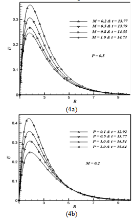 | Figure 4. The simulated steady-state velocity profile at X =1.0 for (a) variation of M ; (b) variation of P |
4.2. Temperature
- The simulated transient temperature (T) for different values of M and P with respect to t is shown at the point (1, 1.15)
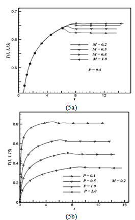 | Figure 5. The simulated transient temperature at (1, 1.15) for (a) variation of M ; (b) variation of P |
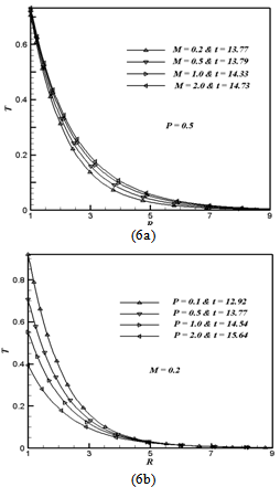 | Figure 6. The simulated steady-state temperature profile at X = 1.0 for (a) variation of M ; (b) variation of P |
4.3. Average Skin-friction Coefficient and Heat Transfer Rate
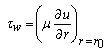
- For engineering purposes, one is usually interested in the values of the skin-friction coefficient and heat transfer rate. The friction coefficient is an important parameter in the heat transfer studies since it is directly related to the heat transfer coefficient. The increased skin-friction is generally a disadvantage in technical applications, while the increased heat transfer can be exploited in some applications such as heat exchangers, but should be avoided in others such as gas turbine applications, for instance. For the present problem these skin-friction coefficient and heat transfer rate are derived and given in the following equations:The wall shear stress at the wall can be expressed as
 | (18) |
 | (19) |
 to be the characteristic shear stress, then the local skin-friction coefficient can be written as
 | (20) |
 | (21) |
 | (22) |
 is given byThus, with the non-dimensional quantities introduced in Eq. (10), Eq. (22) can be written as
 | (23) |
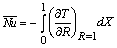 | (24) |
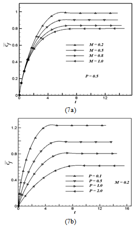 | Figure 7. The simulated average skin-friction for (a) variation of M ; (b) variation of P |
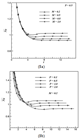 | Figure 8. The simulated average Nusselt number for (a) variation of M ; (b) variation of P |
5. Conclusions
- Conjugate heat transfer analysis on unsteady natural convection hydromagnetic flow of a viscous incompressible fluid over a vertical slender hollow cylinder has been studied. An implicit finite difference scheme of Crank-Nicolson type has been used to solve the governing unsteady, non-linear and coupled equations. The resulting system of equations is solved by using the tridiagonal algorithm. The computations are carried out for different values of magnetic parameter M ( = 0.2, 0.5, 0.8 and 1.0) and conjugate heat transfer parameter P ( = 0.1, 0.5, 1.0 and 2.0). For the velocity and temperature profiles it is observed that the time elapsed to reach the temporal maximum increases with the increasing values of M and P. Time needed to reach the steady-state increases as M and P increases. It is noticed that the velocity and average skin-friction coefficient of the fluid decreases with the increasing values of M. The values of flow variables (U, T) of the fluid decreases as P increases. It is also observed that as P or M increases the steady-state values of average Nusselt number decreases.Nomenclature
 dimensionless average skin-friction coefficientCf dimensionless local skin-friction coefficientCP specific heat at constant pressureg acceleration due to gravityGr Grashof numberH0 applied magnetic fieldkf,ks thermal conductivity of the fluid and the solid cylinder, respectivelyl length of the cylinderM magnetic parameterNu dimensionless average Nusselt numberNuX dimensionless local Nusselt numberP conjugate heat transfer parameterPr Prandtl numberr radial coordinateri,r0 inner and outer radii of the hollow cylinder, respectivelyR dimensionless radial coordinatet′ timet dimensionless timeT0 temperature at the inside surface of the cylinderTS solid temperatureT′ temperature of the fluidT dimensionless temperature of the fluidu, v velocity components in x, r directions respect tivelyU, V dimensionless velocity components in X, R directions respectivelyx axial coordinateX dimensionless axial coordinateGreek Lettersα thermal diffusivityβ volumetric coefficient of thermal expansionρ densityσ electrical conductivity of the fluidμ viscosity of the fluidυ kinematic viscositySubscriptsw conditions on the wall∞ free stream conditions
ACKNOWLEDGEMENTS
- The authors wished to acknowledge support for this research work from the Institute Fellowship (National Institute of Technology Warangal).