Nabil T. M. El-Dabe , M. H. M. Moussa , Rehab M. El –Shiekh , H. A. Hamdy
Department of Mathematics, Faculty of Education, Ain Shams University
Correspondence to: Rehab M. El –Shiekh , Department of Mathematics, Faculty of Education, Ain Shams University.
| Email: |  |
Copyright © 2012 Scientific & Academic Publishing. All Rights Reserved.
Abstract
In this paper, we use two integral methods, the first integral method and the direct integral method to study a higher-order nonlinear Schrödinger equation (NLSE). The application of the first integral method yield trigonometric function solutions and solitary wave solutions. Using the direct integration lead to shock wave solution and Jacobi elliptic function solutions. The direct integral method is more concise and direct than the first integral method.
Keywords:
Higher-Order Nonlinear Schrödinger Equation, the First Integral Method, the Direct Integral Method, Solitary Wave Solutions
1. Introduction
The higher-order nonlinear Schrödinger equation (NLSE) takes the form[1-4]. | (1) |
which describes propagation of ultrashort pulses in nonlinear optical fibers, where the complex function q=q(z,t) is slowly varying envelop of the electric field, the subscripts z and t are spatial and temporal partial derivatives in retard time coordinates also a1, a2, a3, a4 and a5 are the real parameters related to the group velocity, self-phase modulation, third order dispersion, self-steepening and self-frequency shift arising from stimulated Raman scattering respectively see[5-7], some exact solitary wave solutions of Eq. (1) have been successfully obtained by the generally projective Riccat method, the F-expansion method, the extended F-expansion method and -expansion method.The rest of this paper are organized as follow. In section 2, the basic ideas of the first integral method are expressed. In section 3, the method is employed for obtaining the exact solutions. In section 4, we aim using the direct integration on the reduced nonlinear ordinary differential equation obtained after using the travelling wave transformation on the NLSE to get more exact solutions, and finally conclusion is presented in section 5.
2. The First Integral Method
Consider the nonlinear partial differential equation in the from | (2) |
where A=A(x,t) is a solution of the nonlinear partial differential equation (2). We use the transformation | (3) |
where  This enables us to use the following changes:
  | (4) |
Using Eq. (4) to transfer the nonlinear partial differential equation (2) to nonlinear ordinary differential equation | (5) |
Next, we introduce a new independent variable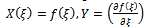 | (6) |
which leads to a system of nonlinear ordinary differential equations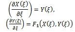 | (7) |
By the qualitative theory of ordinary differential equations[8], if we can find the integrals to Eqs. (7) under the same conditions, then the general solutions to Eqs. (7) can be solved directly. However, in general, it is really difficult for us to realize this even for one first integral, because for a given plane autonomous system, there is no systematic theory that can tell us how to find its first integrals, nor is there logical way for telling us what these first integrals are. We will apply the Division Theorem to obtain one first integral to Eqs. (7) which reduces Eq. (5) to a first order integrable ordinary differential equation. An exact solution to Eq. (2) is then obtained by solving this equation. For convenience, first let us recall the division theorem for two variables in the complex domain C[ω,z].Division Theorem : (see[9-11]) Suppose that P(ω,z) and Q(ω,z) are polynomials in the complex domain C[ω,z]; and P(ω,z) is irreducible in C[ω,z]. If Q(ω,z) vanishes at all zero points of P(ω,z), then there exists a polynomial G(ω,z) in C[ω,z] such that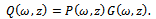 | (8) |
The Divisor Theorem follows immediately from the Hilbert-Nullstenstuz Theorem [12].
3. The Application of the First Integral Method on the (NLSE)
In this section, we study the NLSE using the first integral methodUse the transformation | (9) |
where  is a real function, k, ω and λ are constants, all of them are to be determined.Substituting Eq. (9) into Eq. (1), we obtain an ordinary differential equation for
 ,
, | (10) |
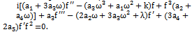
We divide Eq. (10) into two parts imaginary part and real part as follow | (11) |
Re: | (12) |
Integrating Eq. (12), once and setting the integration constants to be zero, then we obtain | (13) |
It can be proved that the following conclusion holds: the necessary and sufficient condition for a non-constant function  satisfying both Eqs. (11) and (13) satisfy the proportional relation as follows:
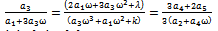 | (14) |
from which it is derived that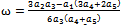 | (15) |
 | (16) |
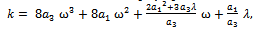
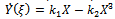
where λ is an arbitrary nonzero constant.Based on the conclusion just mentioned we only solve Eq. (13), instead of both Eqs. (11) and (13), provided that ω and k appearing in Eqs. (11) and (13) are replaced by Eqs. (15) and (16) respectively.For the sake of simplicity we set | (17) |
Then Eq. (13) can be rewritten as a simple form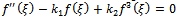 | (18) |
Using (7) we get | (19) |
 | (20) |
According to the first integral method, we suppose that X(ξ) and Y( ξ) are nontrivial solutions of (19), (20) and 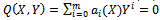 | (21) |
is an irreducible polynomial in the complex domain C[X,Y] such that | (22) |
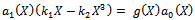
where ai(X) (i=0,1,.......,m), are polynomials of X and am(X)≠0. Eq. (21) is called the first integral to (19), (20). Due to the Division Theorem, there exists a polynomial g(X)+h(X)Y, in the complex domain C[X,Y] such that | (23) |
In this example, we take two different cases, assuming that m=1 and m=2 in (22), we haveCase 1:Suppose that m=1, by comparing the coefficients of  (i=2,1,0) on both sides of (23), we have
 | (24) |
 | (25) |
 | (26) |
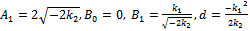
Since ai(X) (i=0,1) are polynomials, then from (24) we deduce that ai(X) is constant and h(X)=0. For simplicity, take a1(X)=1, Balancing the degrees of g(X) and a₀(X), we conclude that deg(g(X))=1 only. Suppose that g(X)=A₁X+B₀, then from (25) we find a₀(X).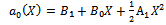 | (27) |
where A₁,B₀ are arbitrary constants , and B₁ is an arbitrary integration constant to be determined.Substituting a₀(X) and g(X) into (26) and setting all coefficients of X powers to be zero, then we obtain a system of nonlinear algebraic equations and by solving it, we obtain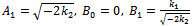 | (28) |
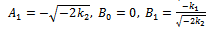 | (29) |
Using conditions (28) in (22), we obtain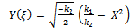 | (30) |
Combining (21) with (19), we obtain the exact solution to (19), (20) and the exact solution to the higher-order nonlinear Schrödinger equation as follows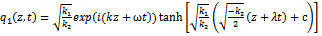 | (31) |
where c is an arbitrary integration constant.Similarly, in the case of (29), from (22), we obtain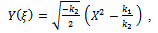 | (32) |
then the exact solution to a higher-order nonlinear Schrödinger equation can be written as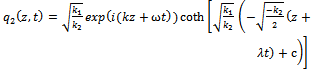 | (33) |
Case 2Suppose that m=2, compare the coefficients of  (i=3,2,1,0) on both sides of (22),we have
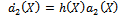 | (34) |
 | (35) |
 | (36) |
 | (37) |
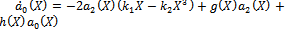
Since ai(X) (i=0,1,2) are polynomials, then from (23) we deduce that a2(X) is a constant and h(X)=0, For simplicity, take a2(X), Balancing the degrees of g(X), a1(X) and a2(X) we conclude that deg(g(X))=1 only. Suppose that g(X)=A1 X+B0, then from (35) and (36) we find a1(X) and a0(X)as follows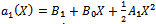 | (38) |
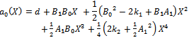 | (39) |
where A1,B0 are arbitrary constants, and B1, d are arbitrary integration constants.Substituting a1(X), a0(X) and g(X) in the last equation in (37) and setting all coefficients of X powers to be zero, then we obtain a system of nonlinear algebraic equations and by solving it with aid of Maple program, we obtain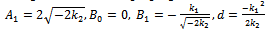 | (40) |
 | (41) |
By using conditions (40) and (41) into (23), we get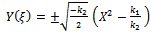 | (42) |
Combining (42) with (19), we obtain the following exact solution to (19),(20) and by back substitution the exact solution to the higher-order nonlinear Schrödinger equation can be written as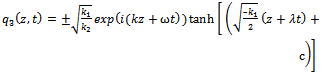 | (43) |
where k1 and k2 appearing in (24)-(43) are expressed by (17), in which ω is expressed by (15).
4. The Direct method
In this section, we multiply Eq. (18) by  , then we get
 | (44) |
Case 1Integrating (44) once and considering the constant of integration to be zero, then we obtain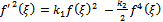 | (45) |
Eq. (45) has the following exact solution by using direct integration method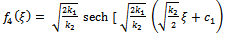 | (46) |
where c1 is an arbitrary integration constant.By back substitution we obtain the following exact solution to a higher-order nonlinear Schrödinger equation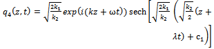 | (47) |
This solutions has been obtained in Ref. [2].Case 2Integrating (44) once then we obtain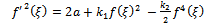 | (48) |
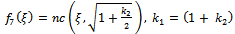
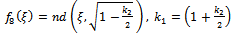
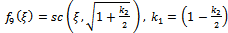
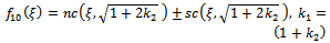
where a is an arbitrary integration constant.Using Jacobi functions, this equation have many solution by relations between values of (2a,  ,) and corresponding f(ξ) see[13], are given by the following
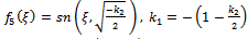 | (49) |
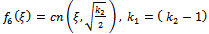 | (50) |
 | (51) |
 | (52) |
 | (53) |
 | (54) |
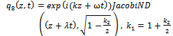
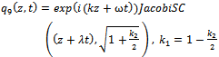
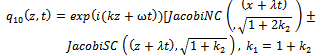
By back substitution we obtain the following new exact solutions to the higher-order nonlinear Schrödinger equation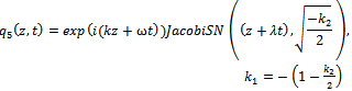 | (55) |
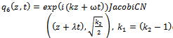 | (56) |
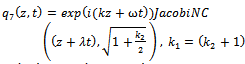 | (57) |
 | (58) |
 | (59) |
 | (60) |
5. Conclusions
In this work, we have obtained many exact solutions of the higher-order nonlinear Schrödinger equation (NLSE) by using the first integral method and the direct method. The application of the two methods was successfully used to establish travelling wave solutions for Eqs. (1). Some of these solutions are different from the results of research in Ref.[1-4], the solution q4(z,t) has been obtained in Ref. [2]. By comparison between the two methods, the direct integral method is easy and powerful than the first integral method.
References
| [1] | Li L.-X., Wang M.-L., Appl. Math. Comput. 208(2009) 440–445. |
| [2] | Hassan M. M., Khater A. H., 387(2008)2433-2442. |
| [3] | Gedalin M., Scott T. C., Band Y. B., Phys. Rev. Lett. 78(1997)448-451. |
| [4] | Zhang J. L., Wang M. L., Li X. R., Chaos Solitons Fract. 33(2007)1450-1457. |
| [5] | Liu C. P., Chaos Solitons Fract. 23 (2005) 949–955. |
| [6] | Xu L. P., Zhang J. L., Chaos Solitons Fract. 31(2007) 937-942. |
| [7] | Abdou M. A., Chaos Solitons Fract. 31(2007) 95–104. |
| [8] | Ding T. R., Li C. Z., Peking University Press, Peking, 1996. |
| [9] | Feng Z., Chaos Solitons Fract. 38 (2008) 481-488. |
| [10] | Zhang T. S., Physics Letters A 371 (2007) 65-71. |
| [11] | Hosseini K., Ansari R., Gholamin P., J. Math. Anal. Appl. 387(2012) 806-814. |
| [12] | N. Bourbaki Commutative Algebra, Addison-Wesley, Paris, 1972. |
| [13] | Yomba E., Chaos Solitons Fract. 27 (2006) 187-196. |
 Abstract
 Reference
 Full-Text PDF
 Full-Text HTML