K. Maleknejad , K. Mahdiani
Department of Applied Mathematics, Islamic Azad University, Karaj Branch, Karaj, Iran
Correspondence to: K. Maleknejad , Department of Applied Mathematics, Islamic Azad University, Karaj Branch, Karaj, Iran.
| Email: |  |
Copyright © 2012 Scientific & Academic Publishing. All Rights Reserved.
Abstract
In this paper, the piecewise constant Block-Pulse functions and their operational matrices of integration have directly been used to solve a two-dimensional Fredholm-Volterra integral equation of second kind. This method presents a computational technique through converting this integral equation into a system of linear equations which can be easily solved by the known methods. Also the error analysis of this method will be considered. The efficiency and accuracy of the proposed method are illustrated by some examples.
Keywords:
Two-dimensional Fredholm-Volterra integral equations, Piecewise constant functions, Block-Pulse functions, Error analysis
Cite this paper:
K. Maleknejad , K. Mahdiani , "Solution and Error Analysis of Two Dimensional Fredholm-Volterra Integral Equations Using Piecewise Constant Functions", American Journal of Computational and Applied Mathematics , Vol. 2 No. 1, 2012, pp. 53-57. doi: 10.5923/j.ajcam.20120201.10.
1. Introduction
Many problems in various fields of science such as physics[1], biology[2] and engineering[3] reduce to integral equations. Integral equations also can be seen in numerous applications such as biomechanics, control, electrical engin- eering, filtration theory, heat and mass transfer, medicine, oscillation theory, etc.[4]. Fredholm-Volterra integral equa- tions of the second kind arise in the studies including airfoil theory[5], elastic contact problems[6,7], fracture mechanics [3], combined infrared radiation and molecular conduction [8] and so on[9]. So, solving these equations specially with higher dimensions is very important. Different methods for solving integral equations have been known and used[9-12].Block-Pulse functions (BPFs), a set of orthogonal functions with piecewise constant values, are studied and applied extensively as a useful tool in the analysis, synthesis, identification as well as other problems of control and systems science. In comparison with other basis functions or polynomials, BPFs can lead more easily to recursive computations in solving concrete problems[13] and among piecewise constant basis functions, the BPFs set has proved to be the most fundamental[14,15]. These functions have been directly used for solving different problems specially integral equations[9,17,18].In this paper, BPFs are applied to estimate the solution of a specific kind of two-dimensional Fredholm-Volterra integ- ral equations  | (1) |
where  ,
,  and
and  are given continuous functions and defined over
  . Also, we consider the error analysis of this method.
2. Block-Pulse functions
We start by repeating some definitions, notations and basic facts; For more details see [13, 16].
2.1. One dimensional Block-Pulse functions
2.1.1. Definition
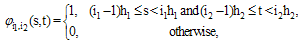
An m-set of BPF's is defined on as 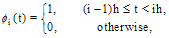 | (2) |
where  , with a positive integer value for
  and
and  .There are some properties for BPF's, the most important properties are disjointness, orthogonality and completeness.
2.1.2.Vector form
The set of BPF's is written as  | (3) |
So, the disjointness property follows 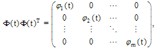 | (4) |
and  | (5) |
where  is an
is an  -vector. Also, for any
  matrix
 | (6) |
where  is a diagonal of matrix
  .
.
2.1.3. BPF's expansion
A function  , can be expanded by BPF's as
 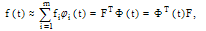 | (7) |
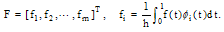 | (8) |
2.1.4.Operational matrix of integration
Integral of  is approximated by the following operational matrix of integration. This matrix is Teoplitze, so it can be used easily.
 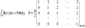 | (9) |
Also, from [13], we have 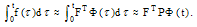 | (10) |
Using (4) gives:  | (11) |
2.2.Two-dimensional Block-Pulse functions
2.2.1. Definition
An  -set of 2D-BPFs is defined in the region of
 | (12) |
where  and
and  with positive integer values for
  , and
, and  Similar to the 1D case, there are some properties for 2D-BPFs such as disjointness, orthogonality and completeness.
2.2.2. Vector form
The set of 2D-BPFs may be written as a -vector 
 | (13) |
where  .
.
2.2.3. BPFs expansion
A function  , can be expanded by BPFs as
 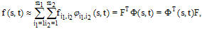 | (14) |
where  is an
is an  -vector given by
 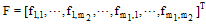 | (15) |
with  | (16) |
Since each 2D-BPF takes only one value in its subregion, they can be expressed by the two 1D-BPFs:  | (17) |
where  and
and  are the 1D-BPFs related to the variables
  and
and  , respectively. From this relation for the function
  , we have
  | (18) |
where  and
and  are
are  and
and  dimensional BPFs vectors respectively, and
  is the
  block-pulse coefficient matrix with
  in (16). In this work, we use (18). It is assumed that
  and so
  Similar to the 1D case, there is an operational matrix of integration for 2D-BPFs. For more details see [18].
3. Direct method for solving 2D-FVIE
In this section, BPFs for solving two-dimensional Fredholm-Volterra integral equations is used. Using the ways mentioned in section 2, the functions  and
and  can be approximated with respect to 2D-BPFs as:
  | (19) |
where the matrices  and
and  are BPFs coefficients of
  and
and  respectively.First, the Volterra integral part in (1) is considered. Using Eq.(19) yields,
 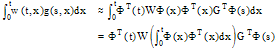 | (20) |
After denoting  for the ith row of the constant matrix
  and
and  for the jth row of the conventional integration operational matrix
  , the relations (4), (5) and (10) give:
 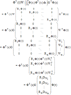 | (21) |
Then, the Fredholm integral part in (1) is considered. The relations (19) and (11) give: 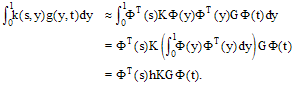 | (22) |
So that (1) can be approximated by 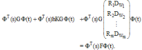 | (23) |
From this equation, the block-pulse coefficients of  can be determined. The jth column of the matrix
  represented by
 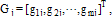 , is obtained by solving jth the system
  | (24) |
where 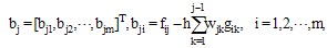 | (25) |
and 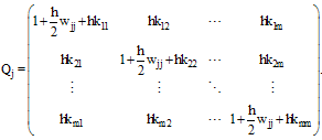 | (26) |
4. Error Analysis
The representation error can be obtained when a differentiable function  is represented in a series of 2D-BPFs over the region
  . We put
 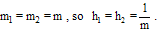 We define the representation error between
  and its 2D-BPFs expansion,
  , over every subregion
  as follows: where Using mean value theorem, it can be shown that
  | (27) |
where  [18]. Representing error between
  and its 2D-BPFs expansion,
  , over the region
  , as follows:
  | (28) |
and using (27), give:  | (29) |
Hence,  . We suppose that
  is approximated by whereas, We find
  -the approximate of
  - and then for
  we have
  | (30) |
Using (29), it can be shown that 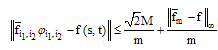 | (31) |
Hence For more details see [18].Now, we consider the following Fredholm-Volterra integral equation of second kind  | (32) |
For an error estimation of Eq.(32), let 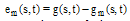 be the error function of the approximate solution
  to
to  , where
  is the true solution of Eq. (32). Substituting the computed solution
  into Eq.(32), the perturbation function that depends only on
  ,
, , can be obtained as follow:
  | (33) |
Subtracting (33) from (32), yields  | (34) |
To compute an approximation of  , Eq.(34) can be solved by the presented method only with recomputing the right hand side of the system (24).
5. Numerical Examples
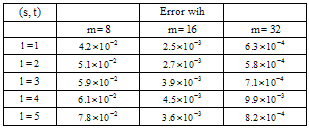
In this section, we use the method discussed of the previous sections for solving some examples. The grid points are selected as  .Example 1. Consider the Fredholm-Volterra integral equation
  | (35) |
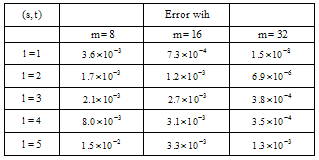
where Exact solution of this equation is  . Table 1 shows the absolute values of error for
  using the present method in selected grid points.
 Table 1. Absolute value of error for Example 1.
 |
| |
|
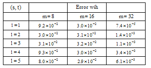
Example 2. The Fredholm-Volterra integral equation  | (36) |
where 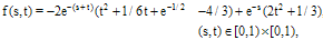 | (37) |
has exact solution  . The numerical results are shown in Table 2.
 Table 2. Absolute value of error for Example 2
 |
| |
|
Example 3. Consider the Fredholm-Volterra integral equation  | (38) |
where 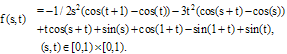 | (39) |
Exact solution of this equation is  . The numerical results are shown in Table 3.
 Table 3. Absolute value of error for Example 3
 |
| |
|
6. Conclusions
Solving analytically two-dimensional integral equations specially a composition of Fredholm and Volterra integral equations is usually complicated and difficult, so using an efficient numerical method make it easy to solve such equations by giving an approximate solution. In the present paper, using piecewise constant functions (BPFs) transformed solving a two-dimensional Fredholm-Volterra integral equation of the second kind to solve systems of linear equations. The advantage of using the above mentioned method is that the elements of the matrices are elements of matrix and they are only different in the elements of main diagonal and this decreases the number of operations. It must be noted that the approximate solution is more accurate at mid-point of every subinterval, and this accuracy will increase as increases. So some points farther to mid-points may get worse as increases. Of course, these oscillations are negligible. This can be clearly followed through the definition of operational matrix . The applicability and accuracy of the method were checked on some examples. The optimal choice of for avoiding accumulated error and increasing the number of operation is important.
References
| [1] | F. Bloom, Asymptotic bounds for solutions to system of damped integro-differential equations of electromagnetic theory, J. Math. Anal. Appl. 73 (1980) 524-542. |
| [2] | K. Holmaker, Global asymptotic stability for a stationary solution of a system of integro-differential equations decribing the formationof liver zones, SIAM J. Math. Anal. 24 (1) (1993) 116-128. |
| [3] | J.R. Willis, Nemat-Nasser, Singular pertubation solution of a class of singular integral equations, Quart. Appl. Math. XLVIII (4) (1990) 741-753. |
| [4] | A.D. Polyanin, A.V. Manzhirov, Handbook of integral equations, 2nd ed., Chapman and Hall/CRC Press, Boca Raton, 2008, Updated, Revised and Extended. |
| [5] | M.A. Golberg, The convergence of a collocations method for a class of Cauchy singular integral equations, J. Math. Appl. 100 (1984) 500-512. |
| [6] | E.V. Kovalenco, Some approximate methods for solving integral equations of mixed problems, Provl. Math. Appl. 103 (3) (1999) 641-655. |
| [7] | B.J. Semetanian, On an integral equation for axially symmetric problem in the case of an elastic body containing an inclusion, J. Appl. Math. Mech. 55 (3) (1991) 371-375. |
| [8] | J. Frankel, A Galerkin solution to regularized Cauchy singular integro-differential equation, Quart. Appl. Math. 52 (2) (1995) 145-158. |
| [9] | C.H. Hsiao, Hybrid function method for solving Fredholm and Volterra integral equations of the second kind, J. Comp. Appl. Math. 230 (1) (2009)59-68. |
| [10] | K. Atkinson, The Numerical Solution of Integral Equatins of the Second Kind, Cambridge university press, 1997. |
| [11] | K. Maleknejad, S. Sohrabi, Y. Rostami, Numerical solution of nonlinear Volterra integral equations of the second kind by using Chebyshev polynomials, Appl. Math. Comp. 188 (2007) 123-128. |
| [12] | K. Maleknejad, T. Lotfi, K. Mahdiani, Numerical Solution of First Kind Fredholm Integral Equations with Wavelets Galerkin Method (WGM) and Wavelets Precondition, Appl. Math. Comp. 186 (2007) 794-800. |
| [13] | Z.H. Jiang, W. Schaufelberger, Block Pulse Functions and Their Applications in Control Systems. Berlin, Springer-Verlag, 1992. |
| [14] | K.G. Beauchamp, Applications of Walsh and Related Functions with an Introduction to Sequency theory, Academic Press, London, 1984. |
| [15] | Deb, G. Sarkar, S.K. Sen, Block pulse functions, the most fundamental of all piecewise constant basis functions, Int. J. Syst. Sci. 25 (2) (1994) 351-363. |
| [16] | E. Babolian, Z. Masouri, Direct method to solve Volterra integral equation of the first kind using operational matrix with block-pulse functions, J. Comp. Appl. Math. 220 (2008) 51-57. |
| [17] | Marzban HR et al. A composition method for the nonlinear mixed Volterra-Fredholm-Hammerstein integral equations. Common Nonlinear Sci Numer Simulat (2010), doi:10.1016/j.cnsns.2010.06.013. |
| [18] | K. Maleknejad, S. Sohrabi, B. Baranji, Application of 2D-BPFs to nonlinear integral equations, Common Nonlinear Sci Numer Simulat, 15 (3) (2010) 528-535. |
 Abstract
 Reference
 Full-Text PDF
 Full-Text HTML