-
Paper Information
- Next Paper
- Previous Paper
- Paper Submission
-
Journal Information
- About This Journal
- Editorial Board
- Current Issue
- Archive
- Author Guidelines
- Contact Us
American Journal of Computational and Applied Mathematics
p-ISSN: 2165-8935 e-ISSN: 2165-8943
2012; 2(1): 46-52
doi: 10.5923/j.ajcam.20120201.09
Numerical Solution of Singularly Perturbed Differential-Difference Equations with Small Shifts of Mixed Type by Differential Quadrature Method
 Abstract
 Reference
 Full-Text PDF
 Full-Text HTML
H. S. Prasad , Y. N. Reddy
Department of Mathematics, National Institute of Technology Warangal-506004, India
Correspondence to: H. S. Prasad , Department of Mathematics, National Institute of Technology Warangal-506004, India.
| Email: |  |
Copyright © 2012 Scientific & Academic Publishing. All Rights Reserved.
In this paper, we have presented the Differential Quadrature Method (DQM) for finding the numerical solution of boundary-value problems for a singularly perturbed differential-difference equation of mixed type, i.e., containing both terms having a negative shift and terms having a positive shift. Such problems are associated with expected first exit time problems of the membrane potential in models for the neuron. The Differential Quadrature Method is an efficient descritization technique in solving initial and/or boundary value problems accurately using a considerably small number of grid points. To demonstrate the applicability of the method, we have solved the model examples and compared the computational results with the exact solutions. Comparisons showed that the method is capable of achieving high accuracy and efficiency.
Keywords: Differential-difference equation; Singular perturbation; Boundary layer; shift; Differential Quadrature Method
Cite this paper: H. S. Prasad , Y. N. Reddy , "Numerical Solution of Singularly Perturbed Differential-Difference Equations with Small Shifts of Mixed Type by Differential Quadrature Method", American Journal of Computational and Applied Mathematics , Vol. 2 No. 1, 2012, pp. 46-52. doi: 10.5923/j.ajcam.20120201.09.
Article Outline
1. Introduction
- A singularly perturbed differential-difference equation is an ordinary differential equation in which the highest derivative is multiplied by a small parameter and involving at least one delay or advance term. In recent papers the terms negative or left shift and positive or right shift have been used for delay and advance respectively. The smoothness of the solutions of such singularly perturbed differential- difference equation deteriorates when the parameter tends to zero. Such problems arise frequently in the study of variational problems of control theory where the problem is complicated by the effect of time delays; this occurs in signal transmission[4] and in depolarization in the Stein model [18], which is a continuous-time, continuous-state space Markov Process whose sample paths have discontinuities of the first kind[10]. The time between nerve impulses is the time of first passage to a level at or above a threshold value; determining the moments of this random variable involves differential-difference equation. The mathematical modelling of the determination of the expected time for generation of action potentials in nerve cells by random synaptic inputs in dendrites includes a general boundary value problem for singularly perturbed differential difference equation with small shifts.The differential-difference equation plays an important role in the mathematical modeling of various practical phenomena in the biosciences and control theory. Any system involving a feedback control will almost always involve time delays. These arise because a finite time is required to sense information and then react to it. For a detailed discussion on differential-difference equation one may refer to the books and high level monographs: Bellen[1], Driver[19], Bellman and Cooke[22]. It is well known that the classical methods fail to provide reliable numerical results for such problems (in the sense that the parameter and the mess size cannot vary independently). Lange and Miura[2-4] gave asymptotic approaches in the study of class of boundary-value problems for linear second-order differential-difference equations in which the highest order derivative is multiplied by small parameter. In [2] and [3], authors pointed out that the shift term can be expanded using a Taylor series, provided the shift is of order ε, with ε small. The effect of small shifts on the oscillatory solution of the problem has been discussed in [3]. In[17], M.K. Kadalbajoo and K.K. Sharma presented a numerical method based on finite difference scheme to solve boundary value problems for singularly perturbed differential-difference equations with small shifts of mixed type. In[16], they described a numerical approach based on finite difference method to solve a mathematical model arising from a model of neuronal variability. In[14], M.K. Kadalbajoo and D. Kumar presented a numerical method based on fitted mess and B-spline technique for singularly perturbed differential-difference equations with small delay. In[15], M.K. Kadalbajoo, D. Kumar, presented a computational method based on piecewise uniform mess and Quasilinearization process for singularly perturbed nonlinear differential-difference equations with small shifts. In[23], M. Gulsu presented matrix methods for approximate solution of the second order singularly perturbed delay differential equations.The aim of this paper is to provide a simple and efficient numerical technique to solve singularly perturbed differential-difference equations of second order with small shifts of mixed type. In this technique, we first approximate the term containing negative/positive shift by Taylor series and then we apply the Differential Quadrature Method (DQM), provided the shifts are of small order of singular perturbation parameter: 𝜺. The DQM approximates the derivative with respect to a coordinate direction at a grid point by a weighted linear sum of all the functional values in that direction. The key to DQM is the determination of weighting coefficients for any order derivative discretization. To the best of the authors knowledge, the Differential Quadrature Method, where approximation of the derivatives have been based on a polynomial of high degree, has not been implemented for the singularly perturbed differential-difference equations of second order with small shifts of mixed type.This paper is organized as follows: Section 2 presents the description of the Differential Quadrature Method, including the formula for finding the weighting coefficients for any order derivative discretization and selection of sampling points. Section 3 presents the basic key procedure to solve differential equation with boundary conditions. Section 4 is devoted to the singularly perturbed differential-difference equations of second order with small shifts of mixed type and its solution procedure by DQM in detail. In the Section 5, we have considered two example problems and presented the Computational results, show the accuracy and efficiency of the method. The conclusions are presented in section 6. The paper ends with the references.
2. Description of the Differential Quadrature Method
- The Differential Quadrature Method (DQM) was introduced by Bellman et al.[20,21] in the early 1970s and, since then, the technique has been successfully employed in finding the solutions of many problems in applied and physical sciences[6-9,11]. The basic idea of differential quadrature method is that the derivative of a function with respect to a space variable at a given point is approximated as a weighted linear sum of the functional values at all discrete points in the domain of that variable.In order to show the mathematical representation of the method, we consider a one dimensional field variable
 prescribed in a field domain
  . Let
. Let  be the function values specified in a finite set of discrete points
  of the field domain. Next, consider the value of the function derivative
  at some discrete points , and let it be expressed as a linearly weighted some of the function values.
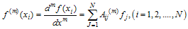 | (1) |
 are the weighting coefficients of the
  -order derivative of the function associated with points
  . Equation (1) the quadrature rule for a derivative is the essential basis of the Differential Quadrature Method. Thus using equation (1) for various order derivatives, one may write a given differential equation at each point of its solution domain and obtain the quadrature analog of the differential equation as a set of algebraic equations in terms of the function values. These equations may be solved, in conjunction with the quadrature analog of the boundary conditions, to obtain the unknown function values provided that the weighting coefficients are known a priori. The weighting coefficients may be determined by some appropriate functional approximations; and the approximate functions are referred to as test functions. The primary requirements for the choices of the test functions are of differentiability and smoothness. That is, the test function of the differential equation must be differentiable at least up to the
  derivative (here
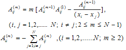
  is the highest order of the differential equation) and sufficiently smooth to be satisfied the condition of the differentiability. Bellman et al.[20] proposed two approaches to compute the weighting coefficients. The first approach solves an algebraic equation system and the second approach uses a simple algebraic formulation, but with the coordinates of grid points chosen as the roots of the shifted Legendre polynomial. Unfortunately, when the order of the algebraic equation system is large, its matrix is ill- conditioned. Thus it is very difficult to compute the weighting coefficients for a large number of grid points. To improve the Bellman’s approaches in computing the weighting coefficients, many attempts have been made by researchers. One of the most useful approaches is the one introduced by Quan and Chang[12,13]. After that Shu’s (Shu[6]) general approach which is based on the high order polynomial approximation and linear vector space analysis, was made available in the literature. This generalized approach computes the weighting coefficients of the first order derivative by a simple algebraic formulation without any restriction on choice of grid points, and the weighting coefficients of second and higher order derivatives by a recurrence relationship.In the DQM, It is supposed that the solution of a one–dimensional differential equation is approximated by a
  terms high degree polynomial:
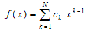 | (2) |
 is a constant.The generalized approach uses two sets of base polynomials to determine the weighting coefficients[6]. The first set of base polynomials is chosen as the Lagrange interpolated polynomials, which are written as Whereandbeing the first derivative of at
  .Here
.Here  are the coordinates of the grid points, can be chosen arbitrarily but distinct.The polynomials
 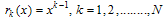 | (4) |
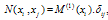 where
where  is the Kronecker operator, the equation (3) is simplified as:
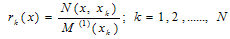 | (5) |
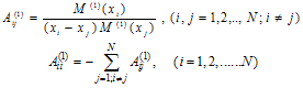 | (6) |
 | (7) |
2.1. Choice of Sampling Points
- A convenient and natural choice for the sampling points is that of the equally spaced points. But the Differential Quadrature solutions usually deliver more accurate results with unequally spaced sampling points. A rational basis for the sampling points is provided by the zeros of the orthogonal polynomials. A well accepted kind of sampling points in the DQM is the so called Gauss-Lobatto- Chebyshev sampling points. For a domain specified by
 and discretized by a set of unequally spaced points (non- uniform grid), then the coordinate of any point
  can be evaluated by:
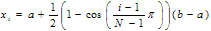 | (8) |
3. Application to Differential Equation
- The basic key procedure in the DQM is to approximate the derivatives in a differential equation by equation (1). Substituting the equation (1) into the governing equations and equating both sides of the governing equations, we obtain simultaneous equations which can be solved by use of Gauss elimination or other methods. That is, DQM is composed of the following procedure:(a) The function to be determined is replaced by a group of function values at a group of selected sampling points. Gauss-Lobatto-Chebyshev sampling points (8) are strongly recommended for numerical stability,(b) Approximate derivatives in a differential equation by these unknown function values.(c) Form a system of linear equations and(d) Solving the system of linear equation yields the desired unknowns.The proper implementation of boundary condition is very important for the accurate numerical solution of differential equation. Essential and natural boundary condition can be approximated by DQM. Using the technique in solving differential equation, the governing equations are actually satisfied at each sampling point of the domain, so one has one equation for each point, for each unknown. In the resulting system of algebraic equation from the DQM, each boundary condition replaces the corresponding field equation. This procedure is straightforward when there is one boundary condition at each boundary and when we have distributed the sampling points so that there is one point at each boundary.
4. Application to Singularly Perturbed Differential-Difference Equations with Small Shifts of Mixed Type
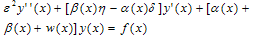
- To show the applicability of DQM, we consider the boundary-value problems for a singularly perturbed differential-difference equation of the mixed type (i.e., containing both terms having a negative shift and terms having a positive shift) with small shifts,
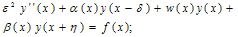 | (9) |
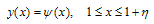
 | (10) |
 | (11) |
 is a singular perturbation parameter,
  and
and  are also small shifting parameters, with
  and
and  The functions
  and
and  are assumed to be sufficiently continuously differentiable functions in The solution to the boundary-value problem (9) with (10) and (11) exhibits the layer behaviour at both ends of the interval
  Since the solution of the boundary-value problem (9) with (10) and (11) is continuous and continuously differentiable on
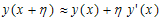
  , so expanding the terms containing shift by Taylor series, we obtain
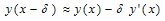 | (12) |
 | (13) |
 | (14) |
 | (15) |
 | (16) |
 ) for the solution of this approximate differential equation. Thus the problem (14) with (15) and (16) results into the following singularly perturbed boundary-value problem:
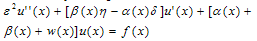 | (17) |
 | (18) |
 | (19) |
 where,
  is the number of sampling/grid points. Denote
 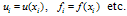 (ii) Apply the DQM to approximate the derivatives in the equation (17), that leads to the following discretized form of the equation:
 | (20) |
 | (21) |
 , that leads to a system of
  equations with
  unknowns.(iv) Use the boundary values for
  and
and  from (21) in the obtained system of equations from step (iii) to get another system of
  equations with
 unknowns
 .(v) Solve the system of equations obtained in step (iv) for the unknowns
  (vi) Use the boundary values to get the complete solution. We have applied the Gaussian elimination method with partial pivoting and employed the double precision Fortran, to solve the obtained system of linear equations in the step (iv), for the unknowns
5. Numerical Illustrations
- To demonstrate the applicability of the DQM, we have applied it to two linear boundary-value problems for a singularly perturbed differential-difference equation of the mixed type (i.e., containing both terms having a negative shift and terms having a positive shift) with small shifts of small order
 In the first example we have considered the problem in which the shift δ is fixed and the shift η is varied. In the second example we have considered the problem in which the shift η is fixed and the shift δ is varied. These examples have been chosen because they have been discussed in literature and because exact solutions are available for comparison. Note that for the considered example problems, the DQM results in the tables, are given in terms of Maximum Absolute Error (M.A.E.) at uniform grids
  , with
  and
and  which have been interpolated through the use of natural cubic spline interpolation polynomial. For the derivation of this polynomial, we have used the DQM results
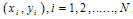 where
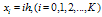
where  are the values of at non-uniform grid points (Gauss-Lobatto-Chebyshev points)
  obtained from (8). To show the accuracy and efficiency of the method with Non-uniform grid points (Gauss-Lobatto-Chebyshev points)
  obtained from (8), we have also given the computational results in terms of Maximum Absolute Error in the tables 5.1(e), 5.1(f), and 5.2(e), 5.2(f), for the example problems- 5.1 and 5.2 respectively, for different values of
  and small parameter:
  .Example 5.1: Consider the following singularly perturbed differential-difference equation with mixed shift from[17]:on [0,1], under the boundary conditionsandFor this example, we have
  The exact solution to this boundary value problem is given by:wherewith The computational results in terms of maximum absolute error for
  are presented in the Tables 5.1(a), 5.1 (b) and for
  are presented in the Tables 5.1 (c), 5.1 (d), for different values of
  and
and  The Maximum Absolute Error in the DQM solution at non-uniform grid points (Gauss-Lobatto-Chebyshev points)
  obtained from (8), with
  and
and  for different values of
  and
and  are presented in the Tables 5.1 (e) and 5.1 (f) respectively.
|
 with
with  for example problem 5.1
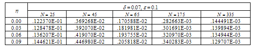
|
 with
with  for example problem-5.1
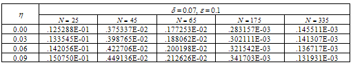
|
 with
with  for example problem-5.1
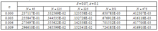
|
 with
with  for example problem-5.1
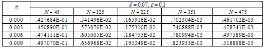
|
 obtained from (8) with different values of
  and
and  , for the example problem-5.1
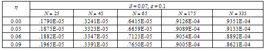
|
 obtained from (8) with different values of
  and
and  , for the example problem-5.1
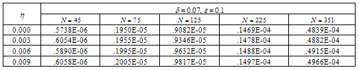
 on [0,1], under the boundary conditionsFor this example, we have
  The exact solution to this boundary value problem has the expression as in Example 5.1 with
  and
and  The computational results in terms of maximum absolute error for
  are presented in the Tables 5.2(a), 5.2 (b) and for
  are presented in the Tables 5.2 (c) , 5.2 (d), for different values of
  and
and  The Maximum Absolute Error in the DQM solution at non-uniform grid points (Gauss-Lobatto-Chebyshev points)
  obtained from (8), with
  and
and  for different values of
  and
and  are presented in the Tables 5.2 (e) and 5.2 (f) respectively.
|
 with
with  for example problem 5.2
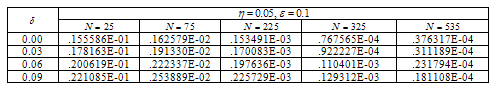
|
 with
with for example problem-5.2
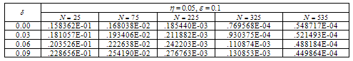
|
 with
with  for example problem-5.2
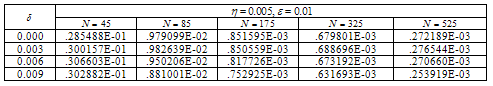
|
 with
with  for example problem-5.2
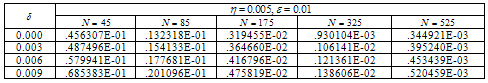
|
 and
and  , for the example problem-5.2
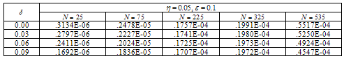
|
 and
and  , for the example problem-5.2
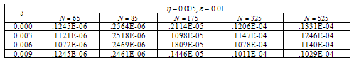
5. Conclusions
- In this paper, we have presented the Differential Quadrature Method (DQM) for finding the numerical solution of linear, second order boundary-value problems for singularly perturbed differential-difference equation of the mixed type (i.e., containing both terms having a negative shift and terms having a positive shift) with small shifts. We have applied the DQM to solve the example problems having both negative and positive shift. The applications presented here showed that the DQM has the capability of solving singularly perturbed differential difference equations with small shifts of mixed type and of producing accurate results with minimal computational effort. We have given here only a few values although the solutions can be computed at desired number of uniform points. It can be observed from the tables that the DQM approximates the exact solution very well with small number of sampling points. This shows the efficiency and accuracy of the present method. It has been observed that an increase in the number of grid points gives rise to an increase in the accuracy of the DQM solution, as in the most numerical techniques. However a small number of grid points in the DQM produces highly accurate results with the use of non-uniform grids. This method provides an alternative technique to the conventional ways of solving singularly perturbed differential-difference equation with small shift of mixed type.
ACKNOWLEDGEMENTS
- The authors are grateful to the reviewers for their valuable suggestions that improve the quality of the paper.