Timo Saksala
Department of Mechanics and Design, Tampere University of Technology, Tampere, P.O. Box 589, FI-33101, Finland
Correspondence to: Timo Saksala , Department of Mechanics and Design, Tampere University of Technology, Tampere, P.O. Box 589, FI-33101, Finland.
| Email: |  |
Copyright © 2012 Scientific & Academic Publishing. All Rights Reserved.
Abstract
It has been observed numerically that the viscoplastic consistency model by Wang (1997) with a linear yield surface and a linear hardening/softening rule converges, using the standard stress return mapping, with two steps. In this paper this numerical observation is proved analytically using the Maple software. The proof is carried out for the Modified Mohr-Coulomb viscoplastic consistency model in the corner plasticity situation, i.e. when both the Rankine and Mohr-Coulomb criteria are violated.
Keywords:
Viscoplastic consistency model, Modified Mohr-Coulomb criterion, Stress return mapping, Exact solution
Cite this paper:
Timo Saksala , "Two-Step Exact Solution for Modified Mohr-Coulomb Viscoplastic Consistency Model with Linear Hardening/Softening: A Proof with Maple Software", American Journal of Computational and Applied Mathematics , Vol. 2 No. 1, 2012, pp. 41-45. doi: 10.5923/j.ajcam.20120201.08.
1. Introduction
The classical viscoplasticity formulations, namely the Perzyna and Duvaut-Lions models, do not utilize the consistency condition[1]. Consequently, trial stress states violating the yield criterion are not returned to the yield surface defined by the yield criterion. In those models, the viscoplastic strain rate depends on the amount of violation[1]. In contrast, the consistency condition is imposed in the more recent viscoplastic consistency model by Wang[2]. Thereby, the trial stresses violating the yield function are returned to the yield surface as in the classical rate- independent plasticity. The major difference to the rate- independent plasticity is the dependence of the yield function on the rate of the internal variable(s). The basic components of the bi-surface viscoplastic consistency model are: 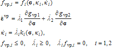 | (1) |
where  denote the internal variable and its rate, respectively. Moreover, gvp,i is the viscoplastic potential,
  is the viscoplastic strain tensor (vector), and
  is the viscoplastic increment, i.e. the rate of viscoplastic multiplier. The yield function fvp,i can be called a dynamic yield function since it can expand and shrink in relation to its static position depending on the loading rate. Moreover, the loading- unloading conditions of Kuhn-Tucker form must hold.As a consequence, the robust stress return algorithms of rate-independent computational plasticity can be employed with minor modifications concerning the presence of the rate of the internal variable(s). It is shown in this paper that a two-step exact solution exists for a viscoplasticity problem with a linear bi-surface yield function and linear hardening/softening laws. This fact has, of course, been observed in numerical simulations but a formal proof is given here. The proof is performed for the Modified Mohr-Coulomb (MMC) viscoplastic consistency model in the corner plasticity situation, i.e. when both the Rankine and Mohr-Coulomb criteria are violated. Moreover, the proof is carried out with the Maple technical computing software due to the complexity of the equations involved. The MMC model is chosen due its wide usage in geotechnical engineering analyses. The MC criterion is usually modified with the Rankine, or the principal stress, criterion to predict the correct tensile strength of geomaterials such as rock and concrete.
2. Modified Mohr-Coulomb Viscoplastic Consistency Model
The MMC yield criterion in the principal stress space, assuming the ordering  , consists of the MC and Rankine criteria:
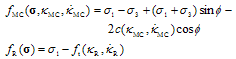 | (2) |
where σ1, σ3 are the major and minor principal stresses, φ is the internal friction, c and ft are the cohesion and tensile strength of the material. The rates of the internal variables are related to viscoplastic increments as 
 with
with 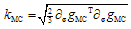 where symbol
 denotes the derivative with respect to a variable (scalar or vector) x. The combined yield surface is illustrated in Figure 1.
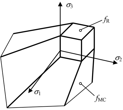 | Figure 1. Modified Mohr-Coulomb criterion in principal stress space |
The rate-dependent softening/hardening rules for cohesion and tensile strength are assumed to be linear by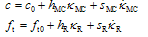 | (3) |
where c0 is the initial (intact) value of cohesion while hMC, hR and sMC, sR are the softening/hardening and viscosity moduli in compression and tension, respectively. In order to account for correct dilatation behaviour of the material in compression, the plastic potential is chosen as | (4) |
where ψ is the dilatation angle. Due to its linearity, the gradients of the MC yield surface and plastic potential are constant vectors (having the angles φ and ψ as parameters). With this choice for the plastic potential, the expression for kMC simplifies as 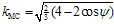 . Therefore, since the relation between the internal variables and plastic increments is a constant relation, it is more convenient to use the plastic multipliers and increments in the following derivations.
 | Figure 2. Illustration of the geometry of a corner point |
3. Return Mapping Scheme for Bisurface Viscoplastic Consistency Model
The intricacy involved in the multisurface plasticity is the stress return to an intersection of yield criteria. At such a point the gradient of the combined yield surface is not unique as illustrated in Figure 2 depicting a corner point in a bi-criteria case.The set of admissible stresses is denoted by Eσ in Figure 1. Γ1 is the region where , in
, in  , and in
  . The stress return algorithm should be able to distinguish between these regions and restore the consistency accordingly. This means, e.g., that if the trial stress lies in Γ1 the single surface integration should be performed in order to return the trial stress to the surface f1 = 0. The determination of the right return can be performed by trial and error only because the condition
  does not guarantee that eventually
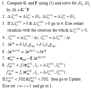
 Here the procedure presented in[3] is employed for determining the active set of yield surfaces.Stress integration, i.e. return mapping, algorithms for classical single and multi-surface plasticity and viscoplasticity are considered, e.g. in[1,3], while algorithms for consistent viscoplasticity are developed in[2,4,5]. For present purposes, the stress integration algorithm by Wang et al.[2] is utilized as modified for the linear bi-surface case. It is assumed that both criteria are violated.Return mapping algorithm for bi-surface viscoplastic consistency model:Compute trial state:
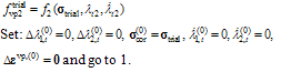 Local iteration:Update:
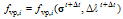
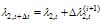 and exit.The expressions for G and F needed in step 1 of the algorithm, derived in Appendix A, are:
 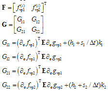 | (5) |
The purpose of step 3 in the algorithm is to ensure that a genuine corner plasticity situation is realized. This can be performed on trial and error only, as noted above. If one of the cumulative plastic increments is found non-positive, the trial stress was located in one of the regions denoted by Γ1 and Γ2 in Figure 2 and, thus, no genuine corner plasticity has occurred (i.e. the trial stress was not located in region Γ12). This means that the bi-surface iteration must be terminated and a single surface integration should be performed to return the trial stress onto the correct yield surface as explained above.In fact, in this form the algorithm above is similar to the generalized cutting plane algorithm[3]. Therefore, it is not limited to linear yield surfaces but can be used for stress integration of nonlinear models as well.
4. A Two-Step Solution for the MMC Viscoplasticity Problem
It is convenient for present purposes to write the MC criterion with its viscoplastic potential in the following simpler form: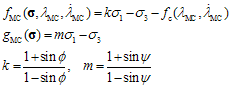 | (6) |
where fc is the uniaxial compressive strength which is substituted for c in Equation (3). In addition, the constant kMC becomes now .Next, it is shown by Maple software that a two-step exact solution, using the algorithm above, exists for the MMC viscoplasticity problem in the corner plasticity situation with the linear hardening/softening rules (3). The proof begins at the onset of viscoplasticity. Vector notation is used and only the relevant intermediate results of the Maple command executions are shown.First time step: transition from elasticity to viscoplasticity, i.e.
 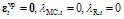 , is treated as shown in Figure 3.
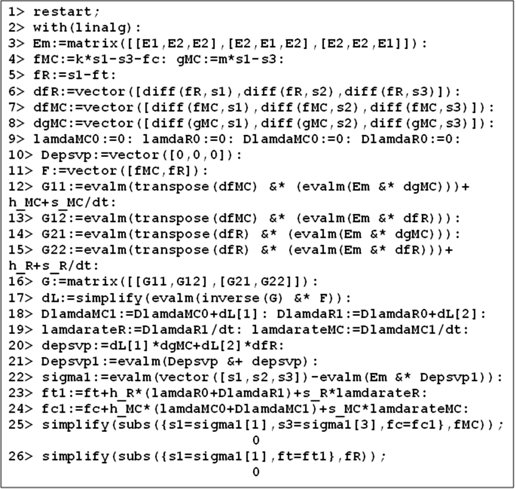 | Figure 3. Maple code for the first iteration involving a transition from elasticity to viscoplasticity |
According to lines 25 and 26 of the Maple code in Figure 3, 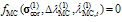 and
and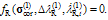 Therefore, at the onset of viscoplasticity, a single step solution exists. Before continuing, the above Maple script is elaborated in some detail. After loading the linear algebra package in line 2, the linear elasticity matrix is defined in line 3 with E1 = E(1−ν)/(1+ν)(1−2ν) and E2 = Eν/(1+ν)(1−2ν) Lines 4-8 define the trial values of the MC and Rankine criteria, the plastic potential (for MC criterion), and their gradients determined with the diff command. In lines 9 and 10 the initial values are set for the viscoplastic multipliers and strain. Vector F and matrix G according to Equation (5) are defined in lines 11-16. Then, the viscoplastic increments are solved in line 17 corresponding to step 1 in the algorithm. Lines 18 and 19 corresponds to steps 2 and 4 in the algorithm. Lines 20 and 21 do the same operations as steps 5 and 6 in the algorithm. Line 22 corrects the stress according to step 7. Lines 23, 24 update the values of uniaxial tensile and compressive strengths and, finally, lines 25 and 26 compute the new values of the yield criteria (step 8 in the algorithm).In the next time step:
 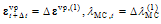 and
and  . This is a general time step involving softening/hardening and the strain rate effects as well. The Maple code is shown in Figure 4.
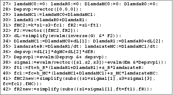 | Figure 4. Maple code for the first iteration involving viscoplasticity |
In line 31 above s1 and s2 denote the trial stress state. Moreover, the Maple commands in lines 41 and 42 yield results that can be written in form: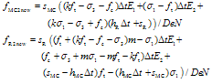 | (7) |
with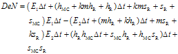 | (8) |
Thus, in the end of the first iteration the values of the yield functions are given by (7). Accordingly, the exact solution is obtained with the first step if the viscosity moduli sMC and sR are set to zero which is the rate-independent case. In the rate-dependent (viscous) case another step is needed: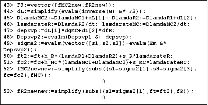 | Figure 5. Maple code for the second iteration involving viscoplasticity |
According to lines 52 and 53 of the Maple code: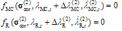 | (9) |
Therefore, only two steps are required for the exact solution which was to be proven.
4. Conclusions
The purpose of this paper was to prove that a two-step exact solution exist for the rate-dependent softening continua modelled with the Modified Mohr-Coulomb viscoplastic consistency model with linear hardening/softening rule. According to the proof with the Maple software, the two-step nature of the consistent viscoplasticity model is located in the invention of the viscosity parameter to the hardening/softening rules. On setting the viscosity modulus to zero, the classical rate-independent MMC plasticity with a single-step exact solution is recovered.Even though the proof was carried out with the MMC model, it can be performed for all other models with linear yield surfaces, such as the Tresca surface, and linear hardening/softening rules.Finally, it has been observed in numerical simulations that also the Drucker-Prager (DP) viscoplastic consistency model with linear hardening/softening rule has the same two-step nature with respect to convergence. This clearly stems from the fact that a closed form solution exists for the rate-independent DP plasticity problem. However, the proof is somewhat more complicated due to the nonlinearity of the DP criterion.
ACKNOWLEDGEMENTS
This research has been funded by Academy of Finland (Grant no. 251626).
Appendix A
The relation for solving the increment of viscoplastic multiplier vector in bi-surface consistent viscoplasticity with linear isotropic hardening/softening laws is derived here. Following notations are used.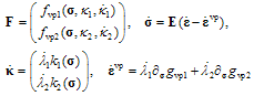 | (A1) |
The yield functions are assumed to be of form 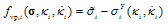 | (A2) |
where is some expression of stress. Yield stresses are assumed to depend linearly on the hardening/softening variables and their rates, i.e.
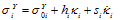 | (A3) |
where hi and si are the constant hardening/softening and viscosity moduli, respectively. At the end of the time step, condition 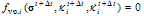 must be satisfied for i= 1,2. Following Winnicki et al.[5], it assumed that
  by which
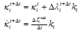 | (A4) |
By (A4) the yield functions fvpi are formulated to depend on :
:  . Hence, F can be expanded with the first term of the vector valued Taylor series:
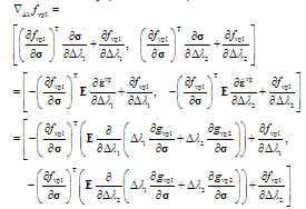 | (A5) |
Computing the gradient of fvp1 with respect to yields (the derivation for fvp2 is identical)
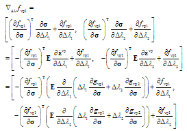 | (A6) |
It is assumed that gvpi is independent of i and f1 is independent of 2. By this, and making use of (A2)-(A4), the first row the gradient (A6) can be written as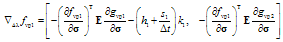 | (A7) |
Now, on solving for and denoting the gradient with G the desired relation is obtained as
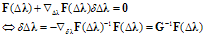 | (A8) |
where G is a 2×2 matrix with the entries in (5).
References
| [1] | Sluys D.R.J, Wave propagation, localisation and dispersion is softening solids, PhD Thesis, Delft University of Technology, 1992. |
| [2] | Wang W.M., Sluys L.J., De Borst R., Viscoplasticity for instabilities due to strain softening and strain-rate softening, International Journal for Numerical Methods in Engineering 1997; 40: 3839-3864. |
| [3] | Simo J.C., Hughes T.J.R., Computational inelasticity, Springer, 1998. |
| [4] | Barpi F., Impact behaviour of concrete: a computational approach. Engineering Fracture Mechanics 2004; 71: 2197-2213. |
| [5] | Winnicki A., Pearce C.J., Bićanić N., Viscoplastic Hoffman consistency model for concrete. Computers & Structures 2001; 79: 7-19. |
 Abstract
 Reference
 Full-Text PDF
 Full-Text HTML