Sh. A. Nazirov , F. M. Nuraliev
Tashkent University of Information Technologies, Uzbekistan, Tashkent
Correspondence to: Sh. A. Nazirov , Tashkent University of Information Technologies, Uzbekistan, Tashkent.
| Email: |  |
Copyright © 2012 Scientific & Academic Publishing. All Rights Reserved.
Abstract
In this work the mathematical model of processes of electro-magnetic fields’ effects on thin conducting plates by complex form, calculating algorithm mining by the joint using variation method and analytical method RFM and software for this algorithm and so calculating experiment are given
Keywords:
Mathematical Modeling, Magneto-Elastisity, Thin Plates
Cite this paper:
Sh. A. Nazirov , F. M. Nuraliev , "Mathematical Modeling of Processes of Electro-Magnetic Fields’ Effectson Thin Conducting Plates by Complex Form", American Journal of Computational and Applied Mathematics , Vol. 2 No. 1, 2012, pp. 30-33. doi: 10.5923/j.ajcam.20120201.05.
1. Introduction
Constructions, machines and devices elements which are in electromagnetic fields of variousorigins are widely applied in modern technic, physics and electrical engineering. Particularly, such elements are found in the measuring devices systems, radio engineering, computer science. In most cases elements of such constructions are thinelectro-conductive plates, and for this reason research of electromagnetic fields influence on them is in a great interest.
2. Problem Statement
The plate in the rectangular x1, x2, x3coordinate system is located so, that the median plane of a plate whichcoincides with x1, x2coordinate plane has σhigh electro-conductivity and is in an electro-magnetic field with a small perturbation. For the solution of this task the magneto-elasticity hypothesis of thin bodies is existedand according to tangential components of electric-field vector intensity driven in electromagnetic field plate and normal components of electric-field vector intensity driven in electromagnetic field plate to the plate thickness are constant. Analytically magneto-elasticity hypotheses for an internal problem are expressed like that[1,2]: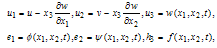 | (1) |
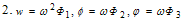
hereu, v,w - deflection of a plate median plane;φ, ψ, f- functions of driven electromagnetic field.In such statement the resolving equations for thin plates in some special cases of an external magnetic field are as follows.[1,2]: | (2) |
here: ε-dielectric constant; μ-magnetic permeability coefficient; c- electro-dynamic constant numerically is equal to the light speed in vacuum; σ-electro-conductivity coefficientof an environment; B0 (B01, B02, B03) - magnetic induction vector for internal area; ρ - platinum material density ; P - external force of non-electromagnetic origin; E- Young model; ν - Poisson's ratio.The equations of magneto-elasticity (2) are solvedat relevant boundary conditions, depended on plate edges fixation technique[1,2]: Rigidly clamped edge of a plate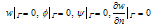 | (3) |
Simply supportededgeof a plate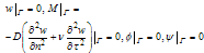 | (4) |
where: n, τ- direction of external normal and tangent to Гborder of a plate and at the given initial conditions: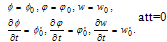 | (5) |
here: φ0, ψ0, w0, φ’0, ψ’0, w’0– accordingly, given at the initial moment of time, where t=0the value of unknown functions and the changes of their speed is zero.The problem of magneto-statics is solved at the first stage of the given problem to defineunknown componentsof B0i magnetic induction for plates magneto-elasticity calculation expressed as the follows: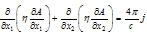 | (6) |
whereFor the equation (6) conditions are defined[3,4]: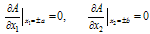 | (7) |
Substituting values of a magnetic induction into equation (2), defined by magneto-statics problem solving (6) - (7)is dynamical problem of thin plates magneto elasticity of complex form.
3. Solution Methods
The problem solution is carried out by Bubnov-Galerkin variation method. At the first stage there have been given the solution structure for the main edge conditions at plate’s complex form by RFM method[5,6]. Let’s demonstrate thesolution structure of the basic boundary conditions (3), (4) and (7). The solution structures for conditions (7),Rigidly clamped edge and Simply supportededges are as follows: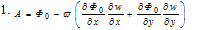 | (8) |
 | (9) |
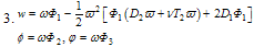 | (10) |
whereHere ω - the normalized equation of plate border, φi, ψi- some full (basic) systems of functions (polynomial function, Chebyshev, trigonometricfunction, etc.), cij- undetermined coefficient of solution structure, definable ;D1, D2, T2 - linear differential operators [5, 6].Substituting (8), (9), (10) solutionstructures in the equation (6) and movements (2), having carried out digitization procedure on spatial variables we will receive resolving equations (discrete model) for a finding of undetermined coefficient of solution structure. In case of statics the resolving equation is represented by system of the linear algebraic equations (SLAE): | (11) |
In case of dynamics the resolving equation is represented by system of the ordinary differential equations (SODE) with initial conditions | (12) |
With initial conditions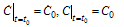 | (13) |
where: M, B - accordingly matrixes of weights and rigidity; F - a vector of the right part; C - a vector of indeterminate components.For the solution of the resolving equations (11) and (12)-(13) it is possible to use known numerical methods of algebra and the analysis, particularly, for the solution of (11) - Gaussian elimination method[7,8], and for the solution(12)-(13)-Newmarkmethod[7,9]. Thus calculation of certain integrals representing components for weight and rigidity matrixes is quite applicable Gaussian double integrals calculation numerical method.
4. The Software
Appropriate software representing a program complex is created on the basis of the developed computing algorithm. The given program complex consists of several modules: for formation of the geometrical information, i.e. for the equations of geometry of areas, their derivatives; for formation of the analytical information, in particular for definition of sub integral expressions; for calculation of solution structure, i.e. for structural formulas; for formation of elements of matrixes of the resolving equations, in particular realization of Gaussian method and so on; formation of points and scales cubature formulas for calculation of integrals; realization of the basic constructive means of R-functions theory, particularly calculation of value of the basic R-operations, differential operators; for solution of the resolving equations, in particular, for the solution of SLAE –Gaussianelimination method, for the decision SODE–Newmarkmethod, calculations of value of basic polynomial, for example power function, trigonometric, Chebyshev; for registration of results of calculation, i.e. construction of tables of decisions, schedules of isolines.
5. Computing Experiment
The difficult form of area of a plate is considered in the form of a rectangle with the approximated corners.The normalized equation of the given area is as follows [5,6]: At carrying out of computing experiment as initial data at the solution of problems are chosen: а=1 m, b=0.5 m (the rectangle party), r=0.1m (radius of a rounding off of corners of a plate) (rice 2.), h=0.01 m, Е=7.1*1011 Н/м2 (the elasticity module), ν =0.3 (Poisson ratio), μ =0.001 Gn/m (magnetic permeability), σ =5.3*1017 (Ohm)-1 (electroconductivity), ε =1 (dielectric permeability), с=3*108 km/s; j=0.01 А/м2, ρ =8890 kg/m3 (copper density). Let's notice, that in the given work we will not stop on the problem solution magnetostatics since it has been in detail enough resulted in the work[11].Results of numerical calculations are more low resulted. In tables 1-2 are resulted a plate bend at action only mechanical forces (fur) and at action of electromagnetic and mechanical forces in characteristic points (0; 0) and (0,5; 0,5) areas, under above resulted boundary conditions, during time moments t changes from 0 to Т with step 0.4 sec, Т=4 sec| Table 1. Plate deflections in the is Rigidly clamped boundary condition |
| | t | w * (x1, x2, t) | | | mech | magn | mech | magn | | (х1,x2) | (0,5; 0,5) | (0,5; 0,5) | (0; 0) | (0; 0) | | 0,4 | 0,001436 | 0,001416 | 0,003763 | 0,003961 | | 0,8 | 0,003498 | 0,003598 | 0,004353 | 0,004052 | | 1,2 | 0,008726 | 0,008822 | 0,003020 | 0,003035 | | 1,6 | 0,009205 | 0,009006 | 0,001734 | 0,009348 | | 2 | 0,002423 | 0,002523 | 0,001230 | 0,002204 | | 2,4 | 0,001369 | 0,001379 | 0,003474 | 0,004841 | | 2,8 | 0,000744 | 0,000745 | 0,001726 | 0,001926 | | 3,2 | 0,003744 | 0,001384 | 0,004039 | 0,000196 | | 3,6 | 0,004246 | 0,004348 | 0,000393 | 0,000193 | | 4 | 0,008445 | 0,008745 | 0,003758 | 0,002881 |
|
|
| Table 2. Plate deflections in Simply supportedboundary condition |
| | | w * (x1, x2, t) | | t | mech | magn | mech | magn | | (х1,x2) | (0,5; 0,5) | (0,5; 0,5) | (0; 0) | (0; 0) | | 0,4 | 0,004739 | 0,001416 | 0,009339 | 0,003465 | | 0,8 | 0,005785 | 0,001598 | 0,001127 | 0,009181 | | 1,2 | 0,002987 | 0,002822 | 0,004875 | 0,002277 | | 1,6 | 0,003451 | 0,009006 | 0,006265 | 0,002366 | | 2 | 0,006448 | 0,000252 | 0,001284 | 0,007437 | | 2,4 | 0,001121 | 0,001379 | 0,008736 | 0,003536 | | 2,8 | 0,002116 | 0,000745 | 0,007288 | 0,002486 | | 3,2 | 0,006665 | 0,001384 | 0,006334 | 0,003413 | | 3,6 | 0,002307 | 0,004348 | 0,004020 | 0,009672 | | 4 | 0,009565 | 0,008745 | 0,002669 | 0,002091 |
|
|
Analyzing the numerical results received at calculations resulted in tables 1-2 it is possible to consider, that magnetic field action is observed owing to influence Lorentz's forces, and is considerable under Simply supportedboundary condition.Further numerical results of calculation a component of the induced electromagnetic field φandψ are resulted at a time interval t = [0; 4]; ∆t = 0,4, accordingly in the same characteristic points of area (tab. 3-4).| Table 3. Components of the induced electromagnetic field |
| | t | Rigidly clamped edge | Simply supported edge | | | φ (0; 0) *103 | ψ (0; 0) *103 | φ (0; 0) *103 | ψ (0; 0) *103 | | 0,8 | -0,001647 | 0,002342 | 0,009886 | 0,001532 | | 1,2 | -0,001044 | 0,005848 | -0,004954 | -0,002337 | | 1,6 | -0,001900 | 0,001096 | -0,004294 | 0,003012 | | 2 | 0,000742 | -0,009653 | -0,002301 | 0,007080 | | 2,4 | 0,003971 | -0,004275 | -0,002157 | -0,002054 | | 2,8 | -0,001273 | 0,001538 | 0,007615 | 0,009546 | | 3,2 | -0,001418 | 0,002546 | 0,002834 | 0,002586 | | 3,6 | -0,002003 | 0,002413 | -0,0005429 | 0,002042 | | 4 | 0,005127 | -0,001001 | -0,0003167 | -0,001475 |
|
|
| Table 4. Components of the induced electromagnetic field |
| | t | Rigidly clamped edge | Simply supported edge | | | φ (0,5; 0,5) *103 | ψ (0,5; 0,5) *103 | φ (0,5; 0,5) *103 | ψ (0,5; 0,5) *103 | | 0,8 | -0,008011 | 0,007680 | -0,000119 | 0,000108 | | 1,2 | -0,003958 | 0,004356 | 0,000169 | -0,000165 | | 1,6 | -0,001917 | 0,002547 | -0,000109 | 0,000111 | | 2 | 0,006445 | -0,006283 | -0,000220 | 0,000219 | | 2,4 | 0,005815 | -0,005952 | 0,000322 | -0,000314 | | 2,8 | -0,004554 | 0,004165 | -0,000510 | 0,000473 | | 3,2 | -0,001110 | 0,001041 | -0,000207 | 0,000207 | | 3,6 | -0,007164 | 0,007018 | 0,000206 | -0,000206 | | 4 | 0,007322 | -0,007050 | -0,000254 | 0,000171 |
|
|
Thus, it is possible to notice, that here magnetic field parametres varies very quickly in relation to a deflection w, have high frequencies and small amplitudes, a field component φ opposite varies under the relation a component ψ.
References
| [1] | Ambarcumyan S.A., Bagdasaryan G.Е., Belubekyan M.V. Magnitouprugosttonkihobolochek i plastin. - M.: Nauka, 1977. - 272 s |
| [2] | Ambarcumyan S.A., Bagdasaryan G.Е., Belubekyan M.V. K magnitouprugostitonkihobolochek i plastin. // PMM. - Moskva, 1973. - T. 37. - Vip. 1. - S. 115-130 |
| [3] | Bins K., Laurenson P. Analiz i raschetelektricheskih i magnitnihpoley. - M.: Energiya, 1970. - 376 s |
| [4] | Ilin V.P. Chislenniemetodiresheniyazadachelektrofiziki. - M.: Nauka,1985 - 336 s |
| [5] | Rvachev V. L., Kurpa L. V. R-funksi v zadachahteoriiplastin. - Kiev: Naukovadumka, 1987. - 176 s |
| [6] | Rvachev V.L. Teoriya R-funksiy i nekotorieeyoprilojeniya. - Kiev: Naukovadumka, 1982. - 552 s |
| [7] | Bate K, VilsonЕ. Chislenniemetodianaliza i metodkonechnihelementov- M.: Stroyizdat, 1982. - 448 s |
| [8] | Fadeev D.K., Fadeeva V.N. Vichislitelniemetodilineynoyalgebri. - M.: Fizmatgiz, 1963. - 734 s |
| [9] | Obraztsov I.F., Savelyev L.M., Hazanov H.S. Metodkonechnihelementov v zadachahstroitelnoymehanikiletatelnihapparatov. M.: Visshayashkola, 1985. - 392 s |
| [10] | Aytmuratov B.SH. Reshenienekotorihzadachmagnitostatikimetodom R - funksiy // Problemiinformatiki i energetiki. - Tashkent, - 2004. № 3. - C. 28-34 |
 Abstract
 Reference
 Full-Text PDF
 Full-Text HTML