Awoke Andargie
Bahir dar University, Department of Mathematics, P.O.Box 79, Bahirdar, Ethiopia
Correspondence to: Awoke Andargie, Bahir dar University, Department of Mathematics, P.O.Box 79, Bahirdar, Ethiopia.
| Email: |  |
Copyright © 2012 Scientific & Academic Publishing. All Rights Reserved.
Abstract
Fitted fourth order central difference scheme is presented for solving singularly perturbed two-point boundary value problems with the boundary layer at one end point. A fitting factor is introduced in a tri-diagonal finite difference scheme and is obtained from the theory of singular perturbations. Thomas Algorithm is used to solve the system and its stability is investigated. To demonstrate the applicability of the method, we have solved linear and nonlinear problems. From the results, it is observed that the present method approximates the exact solution very well.
Keywords:
Singular Perturbation Problems, Finite Differences, Fitted Scheme
Cite this paper: Awoke Andargie, Fourth Order Fitted Scheme for Second Order Singular Perturbation Boundary Value Problems, American Journal of Computational and Applied Mathematics , Vol. 2 No. 1, 2012, pp. 25-29. doi: 10.5923/j.ajcam.20120201.04.
1. Introduction
There are varieties of physical processes in which a boundary layer may arise in the solutions for certain parameter ranges. These types of problems may be generally characterized as singular perturbation problems, and the parameter is termed as the perturbation parameter. Detailed theory and analytical discussion on singular perturbation problems, can be referred in Bender and Orsazag[1], Kevorkian and Cole[3], Nayfeh[5-6], O’Mally[7] and Van Dyke[12] and for exponential fitted methods Miller,J.J.H., O’Riordan,E. and Shishkin, G.I.[4], Y.N.Reddy, P.Pramod. Chakravarthy[9] and Reddy Y.N., Awoke A.[10-11].Fitted stable fourth order scheme is presented for solving singularly perturbed two-point boundary value problems with the boundary layer at one end point. A fitting factor is introduced in a tri-diagonal finite difference scheme and is obtained from the theory of singular perturbations. Thomas Algorithm is used to solve the system and its stability is investigated. To demonstrate the applicability of the method, we have solved several linear and nonlinear problems. From the results, it is observed that the present method approximates the exact solution very well.
2. Fourth Order Finite Difference Method
Consider a linear singularly perturbed two-point boundary value problem of the form:  | (1) |
 | (2a) |
where ε is a small positive parameter (0<ε<<1) and α, β are known constants. We assume that a(x), b(x) and f(x) are sufficiently continuously differentiable functions in[0,1]. Further more, we assume that b(x) ≤ 0, a(x) ≥ M > 0 throughout the interval[0,1], where M is some positive constant. A finite difference scheme is often a convenient choice for the numerical solution of two point boundary value problems, because of their simplicity. Let us divide the interval[0,1] in to N equal parts , each of length h where  and then we have
  . For simplicity, let us denote
  Assuming that y has continuous fourth order derivatives in the interval [0,1], by using Taylor series expansion we obtain the central difference formulas for
  given by.
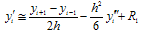 | (3) |
and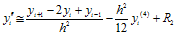 | (4) |
where,  and
and  for
for  .From (1), we have
 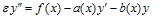 | (5) |
Differentiating both sides of equation (5) with respect to x, we get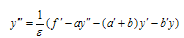 | (6) |
Differentiating twice both sides of equation (5) with respect to x, we get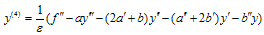 | (7) |
By substituting  from equations (3) and (4) in (1) at
  , we get the central difference approximation in a form that includes all the
  error terms:
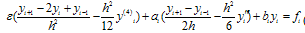 | (8) |
where,  and
and  are defined accordingly in equations (6) and (7) respectively. Using equations (3, 4, 6 & 7) in equation (8), we get the fourth order scheme
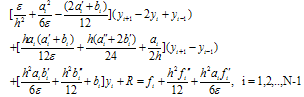 Where,
 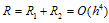 , from equation (4). For detail discussions of the method refer Joshua Y.Choo and David H.Schultz[2].
3. Fitted Fourth Order Scheme
A difference scheme with a fitting factor containing exponential functions is known as exponentially fitted difference scheme. From the theory of singular perturbations it is known that the solution of (1)-(2) is of the form [cf. O’ Malley[7]; pp 22-26]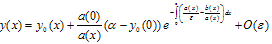 | (9) |
where  is the solution of
 | (10) |
By taking first terms of the Taylor’s series expansion for a(x) and b(x) about the point ‘0’, (10) becomes,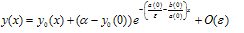 | (11) |
Now we divide the interval [0, 1] into N equal parts with constant mesh length h. Let 0=x0, x1, x2, …xN =1 be the mesh points. Then we have xi = ih; i=0, 1, 2, …, N.From (11) we have 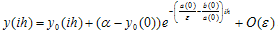 .Therefore
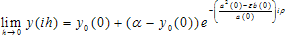 ,Where
 | (12) |
Now, we consider the stable fourth order central difference scheme (8) and introduce the fitting factor :
: | (13) |
Rewriting (13), we have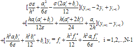 | (14) |
 where σ(ρ) is a fitting factor which is to be determined in such a way that the solution of (14) converges uniformly to the solution of (1)-(2).Multiplying (14) by h and taking the limit as h→ 0; we get
 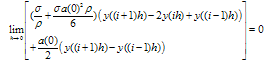 | (15) |
By using (12) in (15) and simplifying, we get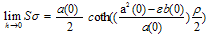 | (16) |
Where | (17) |
We have;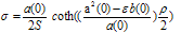 | (18) |
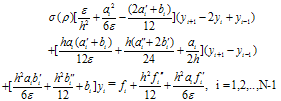
From (14) we have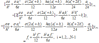 | (19) |
where the fitting factor σ is given by (18).The equivalent three term recurrence relation of equation (19) is given by: | (20) |
where 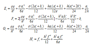 This gives us the tri-diagonal system which can be solved easily by Thomas Algorithm.Thomas AlgorithmA brief discussion on solving the tri-diagonal system using Thomas algorithm is presented as follows: Consider the scheme given in (20):
 subject to the boundary conditions
 | (21a) |
 | (21b) |
We set  | (22) |
where  and
and  which are to be determined.From (22), we have
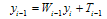 | (23) |
By substituting (23) in (20), we get 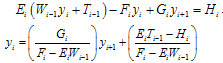 | (24) |
By comparing (24) and (22), we get the recurrence relations | (25a) |
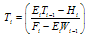 | (25b) |
To solve these recurrence relations for i=0,1,2,3, ,N-1, we need the initial conditions for  and
and  . For this we take
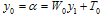 . We choose
  so that the value of
 .With these initial values, we compute
  and
and  for i=1,2,3,….,N-1 from (25) in forward process, and then obtain in the backward process from (22)and (21b).Stability AnalysisWe will now show that the algorithm is computationally stable. By stability, we mean that the effect of an error made in one stage of the calculation is not propagated into larger errors at later stages of the calculations. Let us now examine the recurrence relation given by (25a). Suppose that a small error
  has been made in the calculation of
  ; then, we have
 and we are actually calculating
 | (26) |
From (26) and (25a), we have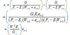 | (27) |
under the assumption that the error is small initially. From the assumptions made earlier that a(x)>0 , b(x)≤0 and its derivatives also non-positive, we have 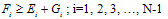 Form (25a) we have
 , since F1>G1
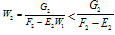 ; since W1 <1,
 ; since F2≥E2 +G2Successively, it follows that
 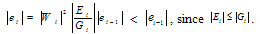 Therefore the recurrence relation (25a) is stable. Similarly we can prove that the recurrence relation (25b) is also stable. Finally the convergence of the Thomas Algorithm is ensured by the condition
  <1, i=1, 2, 3,…., N-1.
4. Numerical Examples
4.1. Example
Consider the following homogeneous singular perturbation problem from Bender and Orszag[[1], page 480; problem 9.17 with α=0]  with y(0)=1 and y(1)=1.The exact solution is given by :
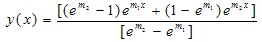 Where
Where 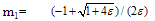 and
and 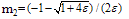 Error plot for Example 4.1, ε=10-3, h=10-2
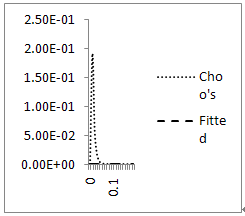 Error plot for example 4.1, ε=10-4, h=10-2.
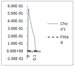
4.2. Example
Let us consider the following non-homogeneous singular perturbation problem from fluid dynamics for fluid of small viscosity, Reinhardt[[8], example 2]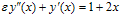 ; x∈[0,1],with y(0)=0 and y(1)=1.The exact solution is given by
 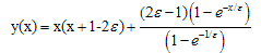 Error plot for Example 4.2, ε=10-3, h=10-2
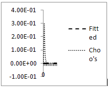 Errorplot for Example 4.2, ε=10-4, h=10-2
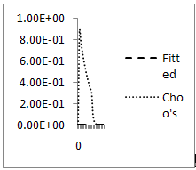
5. Non-linear Problems
Nonlinear singular perturbation problems were converted as a sequence of linear singular perturbation problems by using quasilinearization (Replacing the non-linear problem by a sequence of linear problems) method. The outer solution (the solution of the given problem by putting ε=0) is taken to be the initial approximation.
5.1. Example
Consider the following singular perturbation problem from Bender and Orszag[[1], page 463; equations: 9.7.1] with y(0)=0 and y(1)=0.The linear problem concerned to this example is
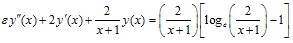 We have chosen to use Bender and Orszag’s uniformly valid approximation[[1], page 463; equation: 9.7.6] for comparison,
 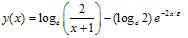 For this example, we have boundary layer of thickness O(ε) at x=0. [cf. Bender and Orszag[1]].Error plot for Example 5.1, ε=10-3, h=10-2
 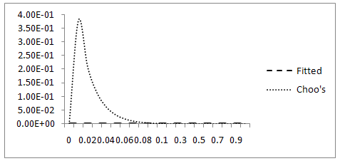 Error plot for Example 5.1, ε=10-4, h=10-2
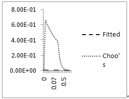
5.2. Example
Let us consider the following singular perturbation problem from Kevorkian and Cole[[3], page 56; equation 2.5.1] 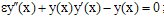 ; x∈[0,1],with y(0)= -1 and y(1)=3.9995The linear problem concerned to this example is
 We have chosen to use the Kevorkian and Cole’s uniformly valid approximation[[3], pages 57 and 58; equations (2.5.5), (2.5.11) and (2.5.14)] for comparison,
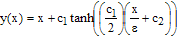 Where c1=2.9995 and c2=(1/c1)loge[(c1-1)/(c1+1)]For this example also we have a boundary layer of width O(ε) at x=0 [cf. Kevorkian and Cole[3], pages 56-66].The numerical results are given in table 4(a), 4(b) for ε=10-3 and 10-4 respectively.Error plot for Example 5.2, ε=10-3, h=10-2
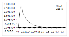 Error plot for Example 5.2, ε=10-4, h=10-2
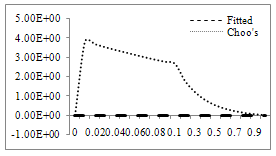
6. Conclusions
We have presented fitted fourth order finite difference method for solving singularly perturbed two-point boundary value problems The present fitted fourth order finite difference method for solving singularly perturbed two-point boundary value problems produce better approximation to the exact solution, specifically in the boundary layer region with step size  , the perturbation parameter.
References
| [1] | Bender, C.M. and Orsazag, S.A.(1978): Advanced Mathematical Methods for Scientists and Engineers, McGraw-Hill, New York |
| [2] | Joshua Y.Choo and David H.Schultz(1993): Stable higher order methods for differential equations with small coefficients for the second order term, Computers Math. Applics: Vol.25,No.1,pp.105-123 |
| [3] | Kevorkian, J. and Cole, J.D. (1981): Perturbation Methods in Applied Mathematics, Springer-Verlag, New York |
| [4] | Miller,J.J.H., O’Riordan,E. and Shishkin, G.I. (1996): Fitted Numerical Methods for Singular Perturbation Problems, World Scientific, River Edge, NJ |
| [5] | Nayfeh A.H. (1981): Introduction to Perturbation Techniques, Wiley, New York |
| [6] | Nayfeh A.H.: Perturbation Methods, Wiley, New York, 1979 |
| [7] | O’Malley, R.E. (1974): Introduction to Singular Perturbations, Academic Press, New York |
| [8] | [8] Reinhardt, H.J. (1980): Singular Perturbations of difference methods for linear ordinary differential equations, Applicable Anal., 10, 53-70 |
| [9] | Reddy Y.N., Chakravarthy P.P. (2004): An exponentially fitted finite difference method for singular perturbation problems, Applied Mathematics and Computation 154, 83-101 |
| [10] | Reddy Y.N., Awoke A. (2007): An Exponentially Fitted Special second order finite difference method for singular perturbation problems, Applied Mathematics and Computation, 190, 1767-1782 |
| [11] | Reddy Y.N., Awoke A. (2007): Fitted fourth order tridiagonal finite difference method for singular perturbation problems, Applied Mathematics and Computation, 192, 90-100 |
| [12] | Van Dyk.M (1964): Perturbation Methods in Fluid Mechanics. Academic Press, New Y (1964): Perturbation Methods in Fluid Mechanics. Academic Press, New York |
 Abstract
 Reference
 Full-Text PDF
 Full-text HTML