Rehab M. El -Shiekh
Department of Mathematics, Faculty of Education, Ain Shams University, Heliopolis, Cairo, Egypt
Correspondence to: Rehab M. El -Shiekh , Department of Mathematics, Faculty of Education, Ain Shams University, Heliopolis, Cairo, Egypt.
| Email: |  |
Copyright © 2012 Scientific & Academic Publishing. All Rights Reserved.
Abstract
In this paper, the variable coefficient two-dimensional Burger equation is studied by two distinct methods. The Exp-function method with the aid of symbolic computation is used to derive soliton solutions of this equation. The  - expansion method is used also to construct travelling wave solutions for the variable coefficient two-dimensional Burger equation with the aid of symbolic computation. The travelling wave solutions are expressed by the hyperbolic, the trigonometric functions and rational functions. The study highlights the significant features of the employed methods and its capability of handling exact solutions for the variable coefficient two-dimensional Burger equation without any restrictions on the form of the variable coefficient. The obtained solutions are considered new with the comparison of other solutions obtained before.
Keywords:
The Exp-function Method; The  - -Expansion Method; The Variable Coefficient Two-Dimensional Burger Equation; New Exact Solutions
Cite this paper:
Rehab M. El -Shiekh , "New Exact Solutions for the Variable Coefficient Two-Dimensional Burger Equation", American Journal of Computational and Applied Mathematics , Vol. 2 No. 1, 2012, pp. 21-24. doi: 10.5923/j.ajcam.20120201.03.
1. Introduction
An evolution equation usually means a partial differential equation with one of the independent variables being time t. There are many nonlinear evolution equations arising from physics, mechanics, biology, chemistry, material science and plasma physics etc. indeed in this paper we confine our attention to the variable coefficients nonlinear evolution equations since they are able to model the real world in many fields of physical and engineering science although their coefficient functions often make the studies very hard also they covers the constant coefficients case by assuming that the coefficient functions constants. One of the variable coefficients nonlinear evolution equations is the variable coefficient two-dimensional Burger equation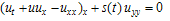 | (1.1) |
Equation (1.1) with s=constant is sometimes referred to as Zabolotskaya-Khokhlov equation in nonlinear acoustics[1,2]. Painlevé analysis of the constant coefficient version of (1.1) was carried out in[3]. The authors showed that the equation possesses the conditional painlevé property and obtained its exact solutions by use of truncation. Also Moussa et al in[4] have applied the symmetry method on Zabolotskaya-Khokhlov equation and obtained new exact solutions for it. Güngӧr in[5-6] used the symmetry method to find similarity reductions for Eq. (1.1) with it's variable coefficient s(t) but those solutions obtained for only some forms of s(t).
2. The Exp-function Method
To illustrate the basic idea of the Exp-function method[7], we consider the following nonlinear evolution equations with only three independent variables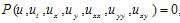 | (2.1) |
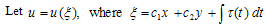
where P is a polynomial function with respect to the indicated variables or some function can be reduce to a polynomial function by using some transformation.Making use of the travelling wave transformation 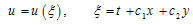 | (2.2) |
Where  and
and  are arbitrary constants to be determined later Then Eq. (2.1) reduces to an ordinary differential equation
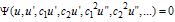 | (2.3) |
The Exp-function method is based on the assumption that the travelling wave solution of the previous equation can be expressed in the following form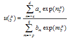 | (2.4) |
where c; d; p and q are unknown positive integers,  and
and  are unknown constants. To determine c and p we balance the linear term of the highest order in (2.3) with the highest order nonlinear term.Similarly, we can determine d and q by balancing the linear term of the lowest order in (2.3) with the lowest order nonlinear term.
3. The  expansion Method
The same assumptions as given before in Eqs. (2.1-2.3) are used but we assume that the solution of Eq. (2.3) takes the following form[8] | (3.1) |
where  satisfy a second order linear differential equation
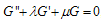 (3.2)where
 and
and  are constants to be determine later. The integer m can be determine by considering the homogeneous balance between the highest derivatives and the highest order nonlinear terms appearing in Eq. (2.3). Then by substituting Eq. (3.1) along with Eq. (3.2) into Eq. (2.3), collecting all terms with the same order of
  together, the left hand side of Eq. (2.3) is converted into another polynomial in
  . Equating each coefficient of this polynomial to zero, yield a set of algebraic equations for
 and
and  which can be solved by using Maple program, along with the general solutions of Eq. (3.1).
4. Solutions of Equation (1.1) by using Exp-function Method
 | (4.1) |
Eq. (1.1) becomes | (4.2) |
Integrate Eq. (4.1) with respect to  twice, we get By re-writing Eq. (2.4) in an alternative form as follows: In order to determine values of c and p, we balance the linear term u′ of the highest order in Eq. (4.3) with the highest order nonlinear term u² and we have
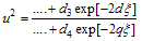
 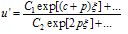 | (4.4) |
 | (4.5) |
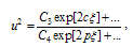
Where  are constant coefficients for simplicity. By balancing the highest order of Exp-function in Eqs. (4.4) and (4.5), we have c + p = 2c, which leads to the limit
 | (4.6) |
Proceeding the same manner as illustrated above, we can determine values of d and q. Balancing the linear term of lowest order in Eq. (4.3)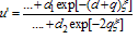 | (4.7) |
 | (4.8) |
where  are determined coefficients only for simplicity, we have - (d + q) = -2d, which leads to results
  | (4.9) |
Case 1. p = c = 1 and d = q = 1, then solution of Eq. (4.3) takes the following form.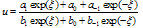 | (4.10) |
By substituting from Eq. (4.10) into Eq. (4.3) and equating the coefficients of the Exp-functions to zero we obtain the following algebraic system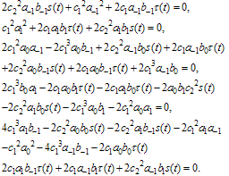 | (4.11) |
Solving the system of algebraic equations (4.11) with the aid of Maple, we obtain by back substitution we get the following new exact solution for the variable coefficient two-dimensional Burger equation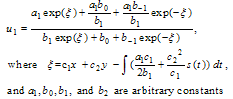 | (4.12) |
Case 2. p = c = 2 and d = q = 1, then Eq. (4.3) has the following solution for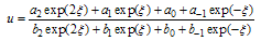 | (4.13) |
Substituting Eq. (4.13) into Eq. (4.3). Equating to zero the coefficients of all powers of  yields a set of algebraic equations for
 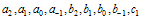 and
and  . Solving this system of algebraic equations with the aid of Maple, we obtain two sets of solutions
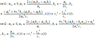 Therefore the variable coefficient two-dimensional Burger equation has the following solitary wave solutions
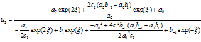 | (4.14) |
where 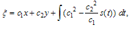 and
and  and
and  are constants.
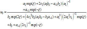 | (4.15) |
where 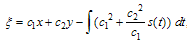 and
and  and
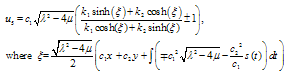
and  are constants.Case 3. p=c=2 and d=q=2, by the same manner as we have done in the previous two cases we obtain the following exact solution for the variable coefficient two-dimensional Burger equation
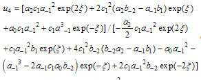 | (4.16) |
Where 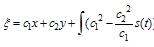 and
and  and
and are constants.
5. New Solutions for Equation (1.1) by using  -expansion Method
By substitution from Eq. (3.1) in (4.3) and balancing the nonlinear term  with the linear
  yield that the leading order m=1, therefore
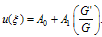 | (5.1) |
By substitution from (5.1) in (4.2) and by using (3.2), then Eq. (4.2) becomes a polynomial in . Equating the coefficients of
  by zero yields the following algebric system
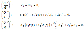 | (5.2) |
Solving the previous system yields the following solutions for it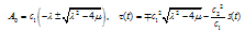 | (5.3) |
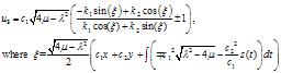
From (5.3) into (5.1) and by using (4.1), we get the following rational and periodic solutions for the variable coefficient two-dimensional Burger equationCase 1: 
 | (5.4) |
If  then we get
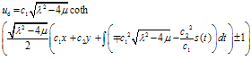 | (5.5) |
Also, if we put  we obtain the following new solution
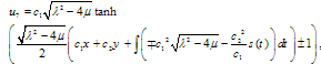 | (5.6) |
Case 2: 
 | (5.7) |
If  then we get
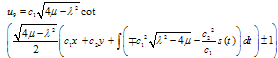 | (5.5) |
Also, if we put  we obtain the following new exact solution
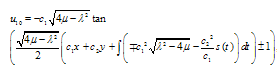 | (5.8) |
In equations from (5.4)-(5.8) are arbitrary constants.
6. Conclusions
In this paper, we have applied the Exp-function method and the  -expansion method on the variable coefficient two-dimensional Burger equation and many new exact solutions in the form of exp-function, hyperbolic, trigonometric functions and rational functions without any restructions on the variable coefficient s(t) which makes those solutions new and not obtained before.
References
| [1] | Zabolotskaya E. A. , Khokhlov R. V. , Sov. phys. Acoust. 15 (1969) 35 |
| [2] | Kuznetsov V. P. , Sov. Pys. Acoust. , 16 (1971) 467 |
| [3] | Webb G. M. , Zank G. P. J. Phys. A: Math. Gen. 23 (1990) 5465 |
| [4] | Moussa M. H. M., El Shikh M. Rehab, Physica A 371 (2006) 325 |
| [5] | Güngӧr F., J. Phys. A: Math. Gen. 34 (2001) 4313 |
| [6] | Güngӧr F., J. Phys. A: Math. Gen. 35 (2002) 1805 |
| [7] | Sheng Zhang, Phys. Lett. A 371 (2007) 65 |
| [8] | Ahmet Bekir, Phys. Lett. A, 372 (2008) 3400 |
 Abstract
 Reference
 Full-Text PDF
 Full-Text HTML