1. Introduction

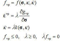
The classical viscoplasticity formulations, namely the Perzyna and Duvaut-Lions models, do not utilize the consistency condition[1]. Consequently, trial stress states violating the yield criterion are not returned to the yield surface defined by the yield criterion. In those models, the viscoplastic strain rate depends on the amount of violation[1]. In contrast, the consistency condition is imposed in the more recent viscoplastic consistency model by Wang[2]. Thereby, the trial stresses violating the yield function are returned to the yield surface as in the classical rate-independent plasticity. The major difference to the rate-independent plasticity is the dependence of the yield function on the rate of the internal variable(s). The basic components of the viscoplastic consistency model are[2]:

(1)

whereare the internal variable and its rate, respectively. Moreover, g_vp is the viscoplastic potential, is the viscoplastic strain tensor (vector), andis the viscoplastic increment. The yield functionf_vp can be calleda dynamic yield function since it can expand and shrink inrelation toits static position depending on the loading rate. Moreover, the loading-unloading conditions of Kuhn-Tucker form must hold.

As a consequence, the robust stress return algorithms of rate-independent computational plasticity can be employed with minor modifications concerning the presence of the rate of the internal variable(s). It is shown in this paper that a two-step exact solution exists for aviscoplasticity problem with a linear yield surface and a linear hardening/softening rule. This fact has been, of course, observed in numerical simulations but a formal proof is given here. The proof is performed for the Mohr-Coulomb (MC) viscoplasticity model with the Maple technical computing software. The MC model is chosen due to its wide usage in geotechnical engineering analyses.

2. Return Mapping Scheme for Viscoplastic Consistency Model

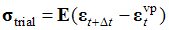
Stress integration, i.e. return mapping, algorithms for classical plasticity and viscoplasticity are considered, e.g. in[1,4], while algorithms for consistent viscoplasticity are developed in[2,4,5]. For present purposes, the stress integration algorithm by Wang et al.[2] is utilized. As all the terms involving the second or mixed derivatives with respect to stress or internal variables disappear due to the linearity (in stress) assumption, the algorithm therein simplifies into a form given below.

Return mapping algorithm for viscoplastic consistency model

Compute trial state: ,

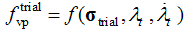
Set: and go to 1.

Local iteration:

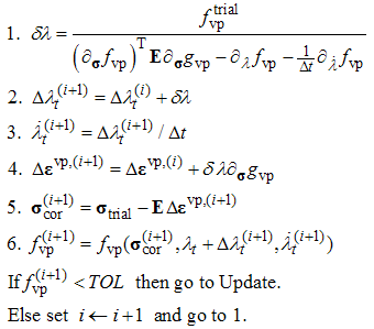Update: ,

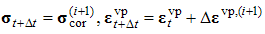and exit.

In the above algorithm symboldenotes the derivative with respect to a variable (scalar or vector) x. Moreover, E denotes the elasticity matrix.

In fact, in this form the algorithm above is similar to the generalized cutting plane algorithm[3]. Therefore, it is not limited to linear yield surfaces but can be used for stress integration of nonlinear models as well.

3. A Two-Step Solution for the MC Viscoplasticity Problem

The MC yield criterion with its viscoplastic potential reads

whereσ₁, σ₃ are the major and minor principal stresses, φ and ψ are the internal friction and dilatation angle, respectively, and c is the cohesion of the material. The rate-dependent softening/hardening rule is assumed linear by

Where c₀ is the initial (intact) value of cohesion while h_MC and s_MC are the softening/hardening and viscosity moduli, respectively. Due to its linearity, the gradients of the MC yield surface and plastic potential are constant vectors (having the angles φ and ψ as parameters).

Next, it is shown by Maple software that a two-step exact solution, using the algorithm above, exists for the MC viscoplasticity problem with the linear hardening/softening rule (3). The proof begins at the onset of viscoplasticity. Vector notation is used and only the relevant intermediate results of the Maple command executions are shown.

First time step: transition from elasticity to viscoplasticity, i.e. , is treated as shown in Figure 1.

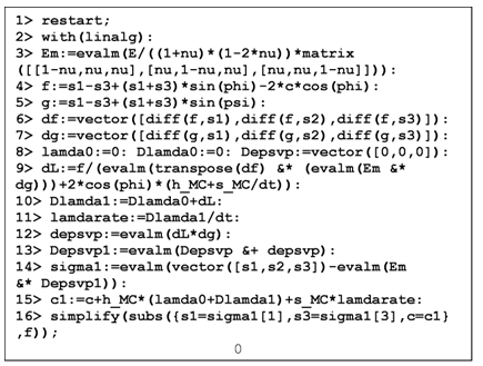Figure 1. Maple code for the first iteration involving a transition from elasticity to viscoplasticity

Thus, . Therefore, at the onset of viscoplasticity, a single step solution exists. Before continuing, the Maple script in Figure 1 is elaborated in some detail. After loading the linear algebra package in line 2, the linear elasticity matrix is defined in line 3. Lines 4-7 define the trial value of the MC yield function, the plastic potential, and their gradients determined with the diff command. In line 8 the initial values are set for the viscoplasticmultiplier and strain. Then, the viscoplastic increment is solved in line 9 corresponding to step 1 in the algorithm. Lines 10 and 11 corresponds to steps 2 and 3 in the algorithm. Lines 12 and 13 do the same operations as step 4 in the algorithm. Line 14 corrects the stress according to step 5. Line 15 updates the value of cohesion and, finally, line 16 computes the new value of the MC yield function (step 6 in the algorithm).

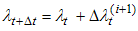
In the next time step: 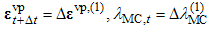. This is a general time step involving softening/hardening and strain rate effects. The Maple code is shown in Figure 2.

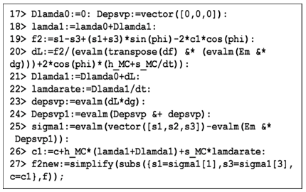Figure 2. Maple code for the first iteration involving viscoplasticity

In line 19 aboves1 and s2 denote the trial principal stress components. Moreover, the Maple command in line 27 yields a result that can be written in form:

Thus, in the end of the first iteration the value of the yield function is given by (4). Accordingly, the exact solution is obtained with the first step if the viscosity moduluss_MC is set to zero which is the rate-independent case. In the rate-dependent (viscous) case another step is needed:

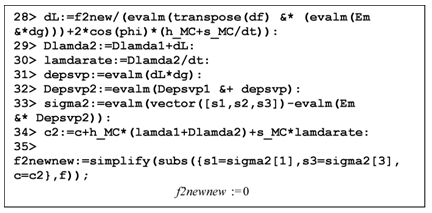Figure 3. Maple code for the second iteration involving viscoplasticity

Thus, . Therefore, only two steps are required for the exact solution which was to be proven.

4. Conclusions

The purpose of this paper was to prove that a two-step exact solution exist for the rate-dependent softening continua modelled with the Mohr-Coulomb viscoplastic consistency model with linear hardening/softening rule According to the proof with the Maple software, the two-step nature of the consistent viscoplasticity model is located in the invention of the viscosity parameter to the hardening/softening rule. On setting the viscosity modulus to zero, the classical rate-independent MC plasticity with a single-step exact solution is recovered.

Even though the proof was carried out with the MC model, it can be performed for all other models with linear yield surfaces, such as the Rankine and Tresca models, and linear hardening/softening rules.

Finally, it has been observed in numerical simulations that also the Drucker-Prager (DP) viscoplastic consistency model with linear hardening/softening rule has the same two-step nature with respect to convergence. This clearly stems from the fact that a closed form solution exists for the rate-independent DP plasticity problem. However, the proof is somewhat more complicated due to the nonlinearity of the DP criterion.