Houssem R. E. H. Bouchekara 1, 2, Mohamed Boucherma 2, Hicham Allag 2, 3
1Department of Electrical Engineering, College of Engineering and Islamic Architecture, Umm Al-Qura University, P. Box: 5555, Makkah, 21955, Saudi Arabia
2Electrical Laboratory of Constantine “LEC”, Department of Electrical Engineering, Mentouri University Constantine, Constantine, 25000, Algeria
3LAMEL Laboratory Jijel University BP 98 Ouled Aissa, Jijel, 18000, Algeria
Correspondence to: Houssem R. E. H. Bouchekara , Department of Electrical Engineering, College of Engineering and Islamic Architecture, Umm Al-Qura University, P. Box: 5555, Makkah, 21955, Saudi Arabia.
| Email: |  |
Copyright © 2012 Scientific & Academic Publishing. All Rights Reserved.
Abstract
An attractive feature of many simulation packages is their availability on desktop computers and their potential for allowing the user to run a simulation model under different conditions in a highly interactive way. Such a way of studying a system is attractive because of its immediacy and the direct control it offers the user. Design of Experiments is a statistical technique for quickly optimizing performance of systems. It starts with a screening experimental design test plan involving all of the known factors that are suspected to affect the system’s performance (or output). When the number of input variables or test factors is large, the primary experimental objective is to pare this number down into a manageable few. This is usually followed by another designed experiment design or test plan with the objective of optimizing the system’s performance. For an easy and interactive use of the design of experiments technique, a new tool called DOET (which stands for ‘Design Of Experiments Tool’) has been developed. This paper aims to illustrate the design of experiments technique using the DOET.In this paper we consider the implementation of the methodology of the design of simulation experiments in the form of interactive tool attached to the simulation model called DOET (which stands for ‘Design Of Experiments Tool’). The DOET receives the output from the simulation model and automatically processes this output using the DOE technique. The DOET thus can be used interactively either to give advice to the user conducting the simulation study, or else to directly control the conduct of the runs.
Keywords:
Design of Experiments, Interactive, Optimal Design, Simulation
Cite this paper:
Houssem R. E. H. Bouchekara , Mohamed Boucherma , Hicham Allag , "Interactive Implementation of Experimental Design Method-Application to Engineering Optimal Design", American Journal of Computational and Applied Mathematics , Vol. 1 No. 2, 2011, pp. 78-85. doi: 10.5923/j.ajcam.20110102.15.
1. Introduction
Engineering Design, in its modern form, is undergoing a transformation from "a process leading to producing a product" to "a product in itself that should be optimally designed". With modern technological advances, products have become more becoming exceedingly complicated. This requires the formation of new design methods and concepts, high performance analysis tools and more powerful optimization/modification algorithms. These techniques now are becoming essential for modern engineering design.As the cost of experimentation rises rapidly it is becoming impossible for the analyst, who is already constrained by resources and time, to investigate the numerous factors that affect these complex processes using trial and error methods[1]. Computer simulations can solve partially this issue. Rather than building actual prototypes, engineers and analysts can build computer simulation prototypes. However, the process of building, verifying, and validating the simulation model can be arduous, but once completed, it can be utilized to explore different aspects of the modelled prototype or device. If the input variables (called also factors) of a process(design and/or optimization) vary, the outputs (responses) causing the majority of the variability in the output? In other words, which factors are the most significant drivers? It is desirable to determine where the variability is coming from (also known as sensitivities) with an optimum utilization of resources[2]. A technique is needed to identify these "vital few" factors in the most efficient manner and then directs the process to meet the desired quality criteria. One extremely effective way for accomplishing this is to use experimental designs, also called Design of Experiments (DOE)[3]. According to[4], many simulation practitioners could obtain more information from their analysis if they use statistical theories, especially with the use of DOE.Compared to one-factor-at-a-time experiments, i.e. only one factor is changed at a time while all the other factors remain constant, the DOE technique is much more efficient and reliable. Though, the one-factor-at-a-time experiments are easy to understand, they do not tell how a factor affects a product or process in the presence of other factors[1]. If the effect of a factor is altered, due to the presence of one or more other factors, we say that there is an interaction between these factors[1]. Usually the interactions’ effects are more influential than the effect of individual factors[1]. This is because the actual environment of the product or process comprises the presence of many factors together instead of isolated occurrences of each factor at different times. The major drawbacks of one factor at a time method are[5]:Many experiments are needed to study the effects of the input factors.The optimum combination of all the variables is not known.The interactions can also not be known.Conclusions are not clear and may be misleading.One cannot get results for non statistical experiments.Since there is no clear distinction, wrong variables may be studied and data obtained may be insufficient or too much.The DOE methodology ensures that all factors and their interactions are systematically investigated. Therefore, information obtained from a DOE analysis is much more reliable and comprehensive than results from the one-factor-at-a-time experiments that ignore interactions between factors and, therefore, may lead to wrong conclusions[1].Let’s assume, for instance, that we want to optimize an induction motor taking into account, for simplicity, only two factors: the length and the external radius. Thus, the length is the first factor and is denoted by  while the external radius is the second factor and is denoted by
 . Each factor can take several values between two limits, i.e.
  and
and . We desire to study the influence of each of these factors on the system response or output (for example the torque) called Y. The classical or traditional approach is to study the two factors
  and
and , separately. First we put
  at the mean level
  and study the response of the system when
  varies between
  to
to , for example, 4 steps (experiments or simulations) are shown in Figure 1. Similarly, we repeat the same procedure to study the effect of
 . The total number of tests is 8. But, do we have a good knowledge about the system with these 8 experiments. The simple and direct answer to this question is no. To get a better knowledge about the system, we have to mesh the validity domain of the two factors and test each node of this mesh as shown in Figure 1. One experiment at each node of the mesh. In this case, we have to achieve 44 =16 experiments. In this example only two factors are taken into account. If the number of factors increases to 7, for example, the number of tests to be performed rises to
  experiments, which is definitely a time and cost consuming process. Knowing that it is impossible to reduce the number of values for each factor to less than 2, the designer often reduces the number of factors, which leads to incertitude of results. To reduce both cost and time, the DOE is used to establish a design experiment with less number of tests. The DOE, for example, allows identifying the influence of 7 factors with 2 points per variable with only 8 or 12 tests rather than 128 tests with the traditional method[2][4].The advantages of implementing a DOE may be listed as[5]:It is more economical and since many factors can be evaluated simultaneously it is less interruptive.In designs the noise factors cannot be controlled but input factors can be. Thus the output produced is deprived of the noise factors.Since the design is well planned, statistically speaking there is no need for in depth knowledge.When compared to one factor at a time method, fewer experiments are carried out.An easy distinction can be made between the factors (noise and important factors).The conclusions drawn are strong since the designs are balanced.Unlike when the classical method of experimentation, the results are clear and any fact overlooked is indicated.Statistical analyses are more precise with the use of statistical software packages.Using this method many quality and reliability issues have been sorted leading to cost savings.
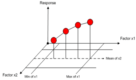 | Figure 1. One experiment at each node of the mesh |
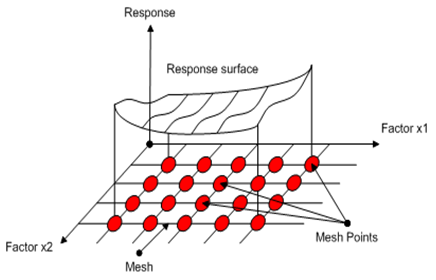 | Figure 2. one experience at each node of the mesh |
Recently, the DOE technique has been adopted in the design and testing of various applications including automotive assembly[6], computational intelligence[7], bioassay robustness studies[8] and many others.The outline of the paper is as follow: this first section constitutes an introduction to the DOE technique. Section 2 explains in detail the methodology of the DOE technique. The implementation of the DOET is described in section 3. The results of applying DOET to some case studies are reported in section 4. Finally, the paper conclusions are provided in Section 5.
2. Methodology
The design and analysis of experiments revolves around the understanding of the effects of different variables on other variable(s)[1]. In terms of mathematical jargon, the objective is to establish a cause-and-effect relationship between several independent variables and a dependent variable of interest[1]. The dependent variable, in the context of DOE, is called the response, and the independent variables are called factors. Experiments are run at different values of the factors, called levels[1]. Each run of an experiment involves a combination of levels of the investigated factors[1]. The number of runs of an experiment is determined by the number of levels being investigated in the experiment. For example, if an experiment involving two factors is to be performed, with the first factor having  levels and the second having
  levels, then
  combinations can possibly be run, and the experiment is an
  factorial design. If all
  combinations are run, then the experiment is a full factorial. If only some of the
  combinations are run, then the experiment is a fractional factorial. In full factorial experiments, all factors and their interactions are investigated, whereas in fractional factorial experiments, certain interactions are not considered. Factorial designs play a fundamental role in the theory and practice of physical experiments. They have been used in a wide range of fields including engineering, social science, agriculture and biology. They allow experimenters to study simultaneously the effects of multiple input variables on the response[9].It can be seen that the size of an experiment escalates rapidly as the number of factors, or the number of the levels, increases. For example, if 2 factors at 2 levels (22) each are to be used, the number of possible combinations for a full factorial design is 22=4. Likewise, for 3 factors at 4 levels (43), the full factorial design has 444=64 experiments. In case of a design where the factors have different number of levels, the determination of the number of experiments is similar. For instance, if we have 3 factors at 2 levels and 2 factors at 4 levels, the full factorial design has 2342=128 experiments. For this reason, many factors are restricted to two levels, and these designs are given a special treatment in this paper. Fractional factorial experiments further reduce the number of treatments to be executed in an experiment as will be explained in the following sections.
2.1. Mathematical Concept
Assume that  is the response (or output) of an experiment (or a simulation) and
 are
are  factors acting on this experiment where each factor has two levels of variation
  and
and . The value of
 , is approximated by an algebraic model given by the following equation:
 | (1) |
where  are coefficients which represent the effect of factors and their interactions on the response of the experiment.
2.2. Full Factorial Design
The study of full factorial design consists of exploring all possible combinations of the factors considered in the experiment[10]. Note that the design  means that this experiment concerns a system with
  factors with
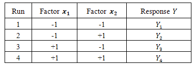
  levels.Usually, two values of the x’s (called levels) are used. The use of only two levels implies that the effects are monotonic on the response variable, but not necessarily linear[2]. For each factor, the two levels are denoted using the "rating Yates” notation (named after its author) by -1 for the low level of each factor and by +1 the high level of each factor (Figure 3). Thus, the number of experiments carried out by a full factorial design with 2 levels is given by:
 | (2) |
where k is the number of factors to be considered. Table 1 shows the design matrix of a full factorial design for 2 factors. Figure 3 sketches the mesh of the experimental field where points correspond to nodes.Table 1. Design Matrix for a full factorial design for 2 factors with 2 levels
 |
| |
|
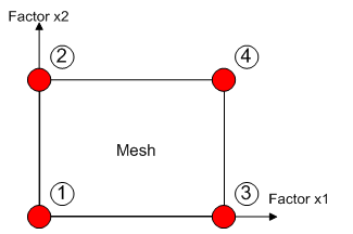 | Figure 3. strategy of experimentation; points corresponding to nodes in the mesh of the experimental field for a full factorial design for 2 factors with 2 levels |
The advantage of full factorial designs, is the ability to estimate not only the main effects of factors, but also all their interactions, i.e. two by two, three by three, up to the interaction involving all k factors. However, when the number of factors increases, the use of such design leads to a prohibitive number of experiments or simulations.The question to be asked is then: is it necessary to perform all experiments of the full factorial design to estimate the system’s response? In other words, is it necessary to conduct a test at each node of the mesh?
2.3. Fractional Factorial Design
A full factorial design consists of all possible treatments. This run size grows rapidly as the number m of factors increases. For example, this run size grows from 32 to 512 as the number of factors increases from 5 to 9. Therefore, running a full factorial design becomes impractical even for a moderately large value of n (runs). Instead, fractional factorial designs are commonly used in practice as they only use a fraction or a subset of the full factorial design[9].It is not necessary to identify the effect of all interactions of the analytical model given by equation (2), because the interactions of order > 2 (like ) are usually negligible. Therefore, certain runs specified by the full factorial design can be used instead of using all runs. To illustrate this phenomenon, an analogy can be made with a Taylor series approximation where the information given by each term decreases if its order increases. So, fractional factorial designs can be used to estimate factors effect and interactions that influence the experiments more with a reduced number of runs[4]. Taguchi Tables[11], or G. Box generators[12], give the fractional factorial design matrix of experiments.To illustrate fractional factorial designs let’s take an example. If the number of factors is
  , the design matrix of these three factors is given by G. Box generators in a way that the third factor is the product of the two other factors. The factor
  and interaction
  are either confused or aliased, and there is a confusion of these aliases because only their sums are reachable[11][13].
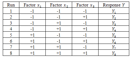
 Table 2. Design Matrix for a full factorial design for 3 factors with 2 levels
 |
| |
|
Table 3. Design Matrix for a fractional factorial design for 3 factors with 2 levels
 |
| |
|
Table 4. G. Box generator of fractional factorial design for 3 factors
 |
| |
|
Table 2 shows a full factorial design for 3 factors with 2 levels. The number of runs is . This number is reduced to 4 using a fractional factorial design as shown in Table 3. As mentioned above the third factor is generated using the G. Box generator for 3 factors given in Table 4. The comparison of the 2 designs is shown in Figure 4.
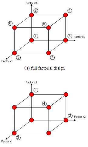 | Figure 4. Comparison between the design experimental field of full and fractional factorial designs with 3 factors |
2.4. Estimation of Model Coefficients
The value of the coefficient  is estimated from the arithmetic average of all observed responses and it is given by:
 | (3) |
where is the response observed for the experiment
  and
and  is the total number of experiments.The effect of a factor
  at the level
  can be calculated thus, the coefficient associated with this effect can be identified using the following equations:
 | (4) |
And | (5) |
where  is the response observed for experiment
  when
when  is at level
 ,
,  is the number of experiments when
  is at level
  and
and  is the effect of coefficient
 .Once the method of how to calculate the coefficients of the model and how to identify the existing confusion between these factors has been presented, we can evaluate the contributions of contrasts (the sum of confusions) and therefore the most significant factors (affecting the response). In[12] the identification of the significant factors has been proposed by evaluating the coefficients contribution (or contrasts, for fractional designs) on the model response from the normalization of their values compared to the sum of squared responses, such as given in the following equations:
 | (6) |
With | (7) |
 | (8) |
where  is the number of levels (equals to 2 in this case),
  is the effect of coefficient
 , and
, and  is the contribution of the contrast associated with the coefficient
 . According to[12]:The contribution given by (6) is deemed significant if
 .The interactions of order higher than two are negligible.If a contrast is negligible, all effects composing this contrast are negligible also.Two significant factors can generate a significant interaction. On the other side, two insignificant factors do not generate a significant interaction.
3. Implementation
For an efficient use of the DOE methodology, it has been implemented in the form of interactive tool the DOET attached to the simulation model. It is a combination of Matlab and Java. Matlab is an efficient software which puts the powerful calculation function, visual and program designing together in an easily used development environment. Java is a cross-platform program development language which is created by Sun. It is the most advanced program language and has the richest characteristic and the most powerful functions. In DOET, Matlab is used for all calculation functions, and java is used to generate interactive User Interfaces.as mentioned earlier the DOET receives the output from the simulation model and automatically processes this output using the DOE technique. The DOET thus can be used interactively either to give advice to the user conducting the simulation study, or else to directly control simulations.When DOET starts, the first window that appears is shown in Figure 5.This is a starting point where the user can mange factors by choosing either options ‘dynamic’ or ‘static’. Dynamic option means that this factor will be considered in the design experiments matrix and will vary between a maximum and a minimum values. The maximum and minimum values of each factor are assigned by the user respectively in the columns ‘Max’ and ‘Min’. Static option means that the factor will not be considered as a varying factor but as a constant and therefore it will not be considered in the design matrix. The values of static factors are assigned by the user in the middle column called ‘Value.’ So the user can set factors and their values to manage the simulation. The user can also choose from the list of ‘functions to be estimated’ which output or answer he/she wants to study. The ‘OK’ button allows running the experiments set in the design matrix. Finally, a sidebar shows the progress of the simulation.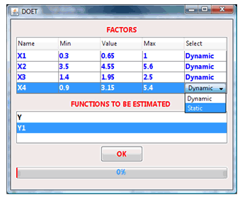 | Figure 5. Main interface of DOET |
4. Applications
4.1. Case Study 1: 3-Factors Ball Bearing Example
The ball and roller bearings consist of an inner race which is mounted on the shaft or journal and an outer race which is carried by the housing or casing. In between the inner and outer race, there are balls or rollers as shown in Figure 6. A number of balls or rollers are used and these are held at proper distances by retainers so that they do not touch each other. The retainers are thin strips and is usually in two parts which are assembled after the balls have been properly spaced. The ball bearings are used for light loads and the roller bearings are used for heavier loads.The life of an individual ball bearing may be defined as the number of revolutions (or hours at some given constant speed) which the bearing runs before the first evidence of fatigue develops in the material of one of the rings or any of the rolling elements.The purpose of this design is to test (under accelerated conditions) new bearing prototypes for use in a specific application for which the current design’s performance was “unsatisfactory”.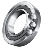 | Figure 6. A Typical Ball Bearing |
The design factors with their levels and types are given in Table 5. The response of interest (y) corresponds to the bearing life (h). The 8 standard runs of the 23 design were randomly ordered, and each prototype bearing tested.| Table 5. Design Factors with their levels and types |
| | Name | Description | Low Level | High Level | Type | | A | Cage Design | Current | New | Discrete | | B | Outer Ring Osculation | Current | New | Discrete | | C | Inner Ring Heat Treatment. | Current | New | Discrete |
|
|
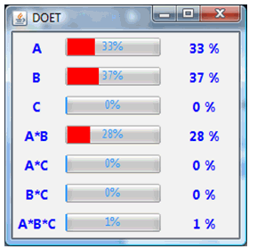
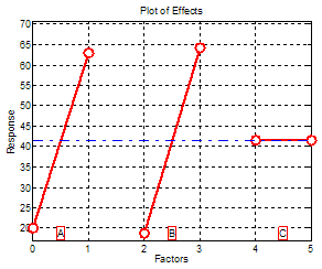
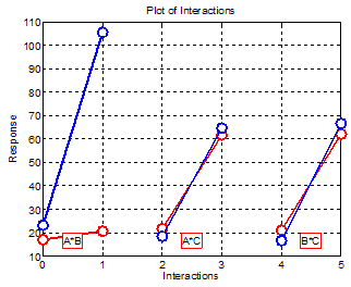
Using the DOET we have investigated this example by generating:The 23 design matrix (see Figure 7). The Contribution obtained. (see Figure 8).The plot of effects given in Figure 9The plot of interactions of factors shown in Figure 10.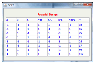 | Figure 7. Design matrix generated by the 23 factorial design and the response or case study 1 |
 | Figure 8. Contribution obtained |
 | Figure 9. Plot of factor effects |
 | Figure 10. Plot of interactions between factors |
From Figure 10 it is evident that to maximize the bearing life the high level of factors A and B must be. The interactions AC and BC are negligible only AB is significative (the lines are not in parallel).Interpretation of the experimentUnexpected Interaction Discovered (Would Not Have Been Discovered Using “One-at-a-Time” Experimentation). Results May Carry Over to Other Bearing Designs.Contrary to Existing Beliefs, the Two Cage Designs had Very Similar Lifetimes. This was Very Important Since Bearings Were Much Cheaper to Produce Under One of the Two Cage Designs.New Design’s Performance (In the Specific Application Under Investigation) Far Superior to That of the Current Bearing Being Used.
4.2. Case Study 2: 6-Factors Switched Reluctance Motor Example
Various advantages of switched reluctance machines and rapid development in the areas of power electronics make them attractive compared to existing DC and AC engines in adjustable speed drives[14]. They have been considered as strong contenders for auxiliary power application in vehicular systems, non-conventional energy sources, and other industrial machineries and equipments[15]. This is owing to their simple and robust construction, fault tolerant capabilities, and extended constant power torque-speed characteristics. They also find application in consumer appliances, such as washing machines and electric bicycles, and they are expected to have growing application in the future[15]. The switched reluctance machine produces torque by the tendency to move its rotor to a position where the inductance of the excited winding is maximized[14]. The construction of the cross-section is very simple and robust because the machine has salient poles on both stator and rotor as shown in Figure 6.Concentrated coils are placed around the stator poles and there are no windings on the rotor, which results in a low rotor inertia and fast dynamic characteristics[14]. The absence of windings and permanent magnets on the rotor and high peak torque-to-inertia ratios makes them well suited for high-speed applications[15].Furthermore, the high power-to-weight and high torque-to-weight ratios of a switched reluctance machine lead to excellent starting characteristics with a high starting torque, a wide speed range as well as a high speed performance[14].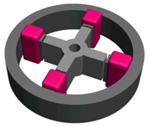 | Figure 11. Geometry of switched reluctance motor |
The purpose of this application is to optimize the geometry of a switched reluctance motor to maximize the magnetic torque exerted by the machine when the rotor is in the position shown in Figure 11[13].This problem can be solved by the finite element method, using a two-dimensional magnetostatic non-linear formulation. Matlab has been used for this purpose.The geometry of the machine is described by seven different geometrical parameters ( ) shown in Figure 11. In our study, only 6 parameters are considered because
  depends on
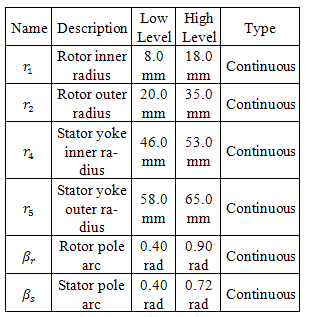
 . The air gap between the rotor and the rotor is constant and equal to 0.25 mm. The limits (or levels) of variation of these parameters were chosen to avoid geometry configuration where the machine is not feasible. These limits are given in Table 6.The objective function of this problem is the Torque T[Nm] exerted by the motor when the rotor is in the desired position.
Table 6. Design Factors with their levels and types
 |
| |
|
4.2.1. Identification of Significant Parameters Using a Fractional Factorial Design
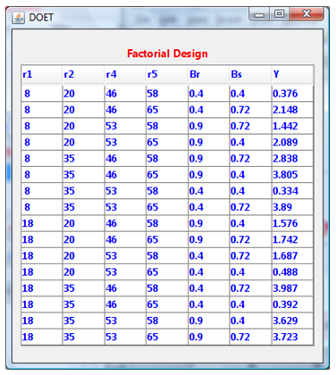
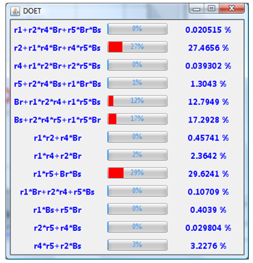
To limit the number of runs or simulations to evaluate the objective function, a 16 experiments fractional design based on the G. Box generators is used here. This design is called a 26-2 fractional factorial design.Using the DOET we have investigated this example by generating:The 26-2 design matrix and the response as shown in Figure 12.The Contrasts and contribution obtained (see Figure 13).The plot of effects given in Figure 14.By analysing the contributions obtained for each parameter, we can conclude that only ,
,  and
and  are significant and influent on the value of the objective function. In addition, we can say that there is a strong interaction between the
  and
and . Therefore, in the optimisation phase only these three parameters are taken into account.
 | Figure 12. Design matrix generated by the 26-2 fractional factorial design and the response or case study 1 |
 | Figure 13. Contrasts and contribution obtained |
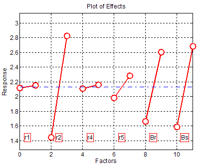 | Figure 14. Plot of factor effects |
5. Conclusions
The approach suggested in this paper is aimed at trying to bridge the gap between existing simulation practice and the substantial design of experiments methodology now available as an interactive tool (DOET) for improving the efficiency of simulation experiments. The development of interfaces like the one described in this paper should enable such desktop use of simulation to become much more efficient and effective.
References
| [1] | ReliaSoft Corporation, 2008, Chapter 2: Overview. Available from: http://www.weibull.com/DOEWeb/experiment_design_and_analysis_reference.htm#introduction.htm>. |
| [2] | M. Uy, J.K. Telford,‘‘Optimization by Design of Experiment techniques’’, IEEE Aerospace conference, Ppp.1-10, March 2009. |
| [3] | Sanchez, S.M. (2005). Work smarter, not harder: guidelines for designing simulation experiments. Proceedings of the Winter Simulation Conference, pp., 4-7. |
| [4] | Bouchekara, H., Dahman, G., Nahas, M. (2011). Smart Electromagnetic Simulations: Guide Lines for Design of Experiments Technique. Progress in Electromagnetics Research B, Vol. 31, 357-379. |
| [5] | Ravikumar, P. Implementation and design issues in large factor experiments. M.S. dissertation, State University of New York at Buffalo, United States -- New York. Retrieved December 4, 2011, from Dissertations & Theses: Full Text.(Publication No. AAT 1456983). |
| [6] | Altayib K., Ali, A. (2011). Improvement for alignment process of automotive assembly plant using simulation and design of experiments. International Journal of Experimental Design and Process Optimization, vol.2, no.2, pp.145-160. |
| [7] | García, S., Fernández, A., Luengo, J. Herrera, F. (2010). Advanced nonparametric tests for multiple comparisons in the design of experiments in computational intelligence and data mining: Experimental analysis of power. Information Sciences, vol.180, no.10, pp. 2044-2064. |
| [8] | Kutlea, L., Pavlovića, N., Dorotića, M., Zadroa, I., Kapustića, M., Halassy, B. (2010). Robustness testing of live attenuated rubella vaccine potency assay using fractional factorial design of experiments. Vaccine, vol.28, no.33, 2010, pp.5497-5502. |
| [9] | Lin, C. New developments in designs for computer experiments and physical experiments. Ph.D. dissertation, Simon Fraser University (Canada), Canada. Retrieved December 4, 2011, from Dissertations & Theses: Full Text.(Publication No. AAT NR58490). |
| [10] | Kleijnen, J. P. C., Sanchez S. M, T.W. Lucas, Cioppa, T. M. (2005). State-of-the-Art Review: A User’s Guide to the Brave New World of Designing Simulation Experiments. Journal on Computing 17(3): 263–289. |
| [11] | M. Pillet, ‘‘Les Plans d’Expériences par la Méthode TAGUCHI’’, Les Editions d’Organisation, ISBN 2-70-812031-X, 1997. |
| [12] | Demonsant, J. (1996). Comprendre et Mener des Plans d’Expériences. Afnor, ISBN 2-124-75032-1. |
| [13] | Costa, M. C. (2001). Optimisation De Dispositifs Electromagnétiques Dans Un Contexte D’analyse Par La Méthode Des Eléments Finis. PhD thesis, National polytechnic institute of Grenoble. |
| [14] | Laudensack, C.; Yu, Q.; Gerling, D., "Investigation of different parameters on the performance of switched reluctance machines," International Conference on Electrical Machines (ICEM), 2010 XIX , vol., no., pp.1-6, 6-8 Sept. 2010. |
| [15] | Desai, P.C.; Krishnamurthy, M.; Schofield, N.; Emadi, A.; , "Switched reluctance machine with higher number of rotor poles for high volume low cost manufacturing," 35th Annual Conference of Industrial Electronics, 2009. IECON '09. IEEE , vol., no., pp.1332-1337, 3-5 Nov. 2009 |

 while the external radius is the second factor and is denoted by
 . Each factor can take several values between two limits, i.e.
  and
and . We desire to study the influence of each of these factors on the system response or output (for example the torque) called Y. The classical or traditional approach is to study the two factors
  and
and , separately. First we put
  at the mean level
  and study the response of the system when
  varies between
  to
to , for example, 4 steps (experiments or simulations) are shown in Figure 1. Similarly, we repeat the same procedure to study the effect of
 . The total number of tests is 8. But, do we have a good knowledge about the system with these 8 experiments. The simple and direct answer to this question is no. To get a better knowledge about the system, we have to mesh the validity domain of the two factors and test each node of this mesh as shown in Figure 1. One experiment at each node of the mesh. In this case, we have to achieve 44 =16 experiments. In this example only two factors are taken into account. If the number of factors increases to 7, for example, the number of tests to be performed rises to
  experiments, which is definitely a time and cost consuming process. Knowing that it is impossible to reduce the number of values for each factor to less than 2, the designer often reduces the number of factors, which leads to incertitude of results. To reduce both cost and time, the DOE is used to establish a design experiment with less number of tests. The DOE, for example, allows identifying the influence of 7 factors with 2 points per variable with only 8 or 12 tests rather than 128 tests with the traditional method[2][4].The advantages of implementing a DOE may be listed as[5]:It is more economical and since many factors can be evaluated simultaneously it is less interruptive.In designs the noise factors cannot be controlled but input factors can be. Thus the output produced is deprived of the noise factors.Since the design is well planned, statistically speaking there is no need for in depth knowledge.When compared to one factor at a time method, fewer experiments are carried out.An easy distinction can be made between the factors (noise and important factors).The conclusions drawn are strong since the designs are balanced.Unlike when the classical method of experimentation, the results are clear and any fact overlooked is indicated.Statistical analyses are more precise with the use of statistical software packages.Using this method many quality and reliability issues have been sorted leading to cost savings.

 levels and the second having
  levels, then
  combinations can possibly be run, and the experiment is an
  factorial design. If all
  combinations are run, then the experiment is a full factorial. If only some of the
  combinations are run, then the experiment is a fractional factorial. In full factorial experiments, all factors and their interactions are investigated, whereas in fractional factorial experiments, certain interactions are not considered. Factorial designs play a fundamental role in the theory and practice of physical experiments. They have been used in a wide range of fields including engineering, social science, agriculture and biology. They allow experimenters to study simultaneously the effects of multiple input variables on the response[9].It can be seen that the size of an experiment escalates rapidly as the number of factors, or the number of the levels, increases. For example, if 2 factors at 2 levels (22) each are to be used, the number of possible combinations for a full factorial design is 22=4. Likewise, for 3 factors at 4 levels (43), the full factorial design has 444=64 experiments. In case of a design where the factors have different number of levels, the determination of the number of experiments is similar. For instance, if we have 3 factors at 2 levels and 2 factors at 4 levels, the full factorial design has 2342=128 experiments. For this reason, many factors are restricted to two levels, and these designs are given a special treatment in this paper. Fractional factorial experiments further reduce the number of treatments to be executed in an experiment as will be explained in the following sections.
 is the response (or output) of an experiment (or a simulation) and
 are
are  factors acting on this experiment where each factor has two levels of variation
  and
and . The value of
 , is approximated by an algebraic model given by the following equation:
 are coefficients which represent the effect of factors and their interactions on the response of the experiment.
 means that this experiment concerns a system with
  factors with
  levels.Usually, two values of the x’s (called levels) are used. The use of only two levels implies that the effects are monotonic on the response variable, but not necessarily linear[2]. For each factor, the two levels are denoted using the "rating Yates” notation (named after its author) by -1 for the low level of each factor and by +1 the high level of each factor (Figure 3). Thus, the number of experiments carried out by a full factorial design with 2 levels is given by:

 ) are usually negligible. Therefore, certain runs specified by the full factorial design can be used instead of using all runs. To illustrate this phenomenon, an analogy can be made with a Taylor series approximation where the information given by each term decreases if its order increases. So, fractional factorial designs can be used to estimate factors effect and interactions that influence the experiments more with a reduced number of runs[4]. Taguchi Tables[11], or G. Box generators[12], give the fractional factorial design matrix of experiments.To illustrate fractional factorial designs let’s take an example. If the number of factors is
  , the design matrix of these three factors is given by G. Box generators in a way that the third factor is the product of the two other factors. The factor
  and interaction
  are either confused or aliased, and there is a confusion of these aliases because only their sums are reachable[11][13].
  . This number is reduced to 4 using a fractional factorial design as shown in Table 3. As mentioned above the third factor is generated using the G. Box generator for 3 factors given in Table 4. The comparison of the 2 designs is shown in Figure 4.
 is estimated from the arithmetic average of all observed responses and it is given by:
 is the response observed for the experiment
  and
and  is the total number of experiments.The effect of a factor
  at the level
  can be calculated thus, the coefficient associated with this effect can be identified using the following equations:

 is the response observed for experiment
  when
when  is at level
 ,
,  is the number of experiments when
  is at level
  and
and  is the effect of coefficient
 .Once the method of how to calculate the coefficients of the model and how to identify the existing confusion between these factors has been presented, we can evaluate the contributions of contrasts (the sum of confusions) and therefore the most significant factors (affecting the response). In[12] the identification of the significant factors has been proposed by evaluating the coefficients contribution (or contrasts, for fractional designs) on the model response from the normalization of their values compared to the sum of squared responses, such as given in the following equations:


 is the number of levels (equals to 2 in this case),
  is the effect of coefficient
 , and
, and  is the contribution of the contrast associated with the coefficient
 . According to[12]:The contribution given by (6) is deemed significant if
 .The interactions of order higher than two are negligible.If a contrast is negligible, all effects composing this contrast are negligible also.Two significant factors can generate a significant interaction. On the other side, two insignificant factors do not generate a significant interaction.


 ) shown in Figure 11. In our study, only 6 parameters are considered because
  depends on
 . The air gap between the rotor and the rotor is constant and equal to 0.25 mm. The limits (or levels) of variation of these parameters were chosen to avoid geometry configuration where the machine is not feasible. These limits are given in Table 6.The objective function of this problem is the Torque T[Nm] exerted by the motor when the rotor is in the desired position.
 ,
,  and
and  are significant and influent on the value of the objective function. In addition, we can say that there is a strong interaction between the
  and
and . Therefore, in the optimisation phase only these three parameters are taken into account.


 Abstract
 Reference
 Full-Text PDF
 Full-Text HTML