Masoud Saravi
Islamic Azad University, Department of Mathematics Nour Branch, Nour, Iran
Correspondence to: Masoud Saravi , Islamic Azad University, Department of Mathematics Nour Branch, Nour, Iran.
| Email: |  |
Copyright © 2012 Scientific & Academic Publishing. All Rights Reserved.
Abstract
In this paper we introduce, briefly, Clenshaw method which is a kind of spectral method and then by exploiting the trigonometric identity property of Chebyshev polynomial in this method we try to get more accurate approximate solution of linear differential equations. We compare the results by some numerical examples.
Keywords:
Clenshaw Method, Pseudo-Clenshaw Method, Chebyshev Polynomials
Cite this paper:
Masoud Saravi , "On the Clenshaw Method for Solving Linear Ordinary Differential Equations", American Journal of Computational and Applied Mathematics , Vol. 1 No. 2, 2011, pp. 74-77. doi: 10.5923/j.ajcam.20110102.14.
1. Introduction
Spectral methods arise from the fundamental problem of approximation of a function by interpolation on an interval, and are very much successful for the numerical solution of ordinary or partial differential equations[1]. Since the time of Fourier (1882), spectral representations in the analytic study of differential equations have been used and their applications for numerical solution of ordinary differential equations refer, at least, to the time of Lanczos[2]. Spectral methods have become increasingly popular, especially, since the development of Fast transform methods, with applications in problems where high accuracy is desired. A survey of some applications is given in[3].The basis of spectral methods to solve differential equations is to expand the solution function as a finite series of very smooth basis functions, as follows  | (1) |
in which,  is one of choice of the eigenfunctions of a singular Sturm-Liouville problem. If the solution is infinitely smooth, the convergence of spectral method is more rapid than any finite power of 1/N. That is the produced error of approximation (1), when
 , approaches zero with exponential rate[1]. This phenomenon is usually referred to as “spectral accuracy”[3]. The accuracy of derivatives obtained by direct, term by term differentiation of such truncated expansion naturally deteriorates[1]. Although there will be problem but for high order derivatives truncation and round off errors may deteriorate, but for low order derivatives and sufficiently high-order truncations this deterioration is negligible. So, if the solution function and coefficientfunctions of the differential equation are analytic on, spectral methods will be very efficient and suitable. We call function y is analytic onif is infinitely differentiable and with all its derivatives on this interval are bounded variation. In next section, first, we introduce Clenshaw method and then by exploiting the trigonometric identity property of Chebyshev polynomial, we develop a numerical scheme referred to as Pseudo-Clenshaw method.
2. Procedures
(i)-Clenshaw methodConsider the following differential equation: | (2) |
 | (3) |
where , and
, and ,
,  , are known real functions of
  denotes
  order of differentiation with respect to
  is a linear functional of rank
  and
and .Here (3) can be initial, boundary or mixed conditions. The basis of spectral methods to solve this class of equations is to expand the solution function,, in (2) and (3) as a finite series of very smooth basis functions, as given below
  | (4) |
where,  is sequence of Chebyshev polynomials of the first kind. By replacing
  in (2), we define the residual term by
  as follows
 | (5) |
In spectral methods, the main target is to minimize  throughout the domain as much as possible with regard to (3), and in the sense of point-wise convergence. Implementation of these methods leads to a system of linear equations with
  equations and
  unknowns
  Consider the following differential equation:
 | (6) |
First, for an arbitrary natural number , we suppose that the approximate solution of equations (6) is given by (4). Our target is to find
 . For this reason, we put
  | (7) |
Using this fact that the Chebyshev expansion of a function  is
is , we can find coefficients
  and
and  as follows:
 | (8) |
where,  and
and  for
for  To compute the right-hand side of (8) it is sufficient to use an appropriate numerical integration method. Here, we use
  - point Gauss - Chebyshev - Lobatto quadrature
  ,where
  and
and  for
for .Note that, for simplicity of the notation, these points are arranged in descending order, namely,
 ,with weights
 and nodes
  That is, we put[4]:
 ,and using
  we get
 where, notation
  means first and last terms become half. Therefore, we will have:
 | (9) |
Now, substituting (4) and (9) in equations (6), and using the fact that
 in this manner, we get
 | (10) |
 | (11) |
Now, we multiply both sides of (10) by , and integrate from -1 to 1, to obtain
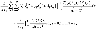 | (12) |
where, | (13) |
with,  ,when
,when , and zero when
  [5].We can also compute the integrals in the right-hand side of (12) by the method of numerical integration using -point Gauss-Chebyshev-Lobatto quadrature. Therefore, substituting (13) in (12) and using the fact that
  equations (12) and (11) make a system of
  equations for
  unknowns
 , and we can obtain
  from this system.(ii)-Pseudo-Clenshaw methodWe assume that an approximate solution to Eq. (6) is given by
 | (14) |
Recall the Chebyshev polynomial given by: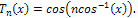 Let
Let , then
 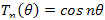 By using this identity (14) becomes
 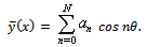 | (15) |
The first and second derivatives of (15) are given, respectively, as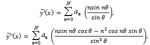 Substituting
  and
and  in Eq. (6) with the functions
  and
and  in term of
 , we get
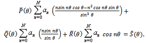 where
where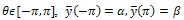 and
and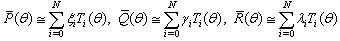 Some more substitutions through 8-13 lead to desire relations.
3. Numerical Examples
Now, we consider some examples with Clenshaw and Pseudo-Clenshaw methods and observe the power of this method comparing with usual numerical methods such as Euler’s or Runge-Kutta’s, Adams methods. Problem 1. Consider with exact solution
 .We solved it by Runge-Kutta with orders two and four and also method. For these methods we used, the same step size and step number. The maximum errors were
 , respectively. We, also, solved it by shooting method with the same step size for steps N=14, 17. We had maximum errors
  respectively. As we see the rate of improvement of accuracy is very low. But we used the Clenshaw method with Chebyshev e basis for
  and
and  .The maximum errors were about,
  , and
, and , respectively, and we used the Pseudo- Clenshaw method with
 , and maximum errors were
 , and
, and , respectively. As we can see, Clenshaw and Pseudo- Clenshaw methods for solving such problems have high rate of convergency. Existence of
 , indicates when N get the value 7, the error becomes zero. If we observe above errors they are rounding errors.Example 2. Let us consider
 with the exact solution
 . This example was chosen from[6]. We solved it by Runge-Kutta with orders two and four and also Adams method. The maximum errors are
 , respectively. That is, these methods give good results for such problems. For these methods we used the same step size and step number. We also solved it by the Clenshaw and Pseudo-Clenshaw methods with
 , the maximum errors produced from this method are given in Table 1, where
  and
and  mean the Clenshaw and Pseudo-Clenshaw methods, respectively.
Table 1.
 |
| |
|
Problem 3: Consider where,
  so that the exact solution is
  For comparison, we solved this problem by finite difference method, using the central differences for the derivatives. The mesh points are given by
 . The maximum errors given by this method are,
 for
for , respectively.We solved it by the Clenshaw and Pseudo-Clenshaw methods with
 , the maximum errors produced from this method are given in Table 2 shows the results of solving this problem by these methods.
Table 2.
 |
| |
|
4. Conclusions
Results in these examples show the efficiency of Pseudo- Clenshaw method for obtaining a better numerical result. Unfortunately, for equations with non-analytical coefficient functions these methods have low convergence, because whenincreases the rate of improvement of accuracy is very low. This is because of the lack of smoothness of the coefficient function. But, when we solved it by the pseudo-spectral method, since coefficient functions do not need expansion in the form of (9), the error produced from using this method, will be better than Clenshaw and Pseudo-Clenshaw methods[6].Author next goal is to work more on this method to get better results.
References
| [1] | C. Canuto, M. Hussaini, A. Quarteroni, T. Zang, Spectral Methods in Fluid Dynamics, Springer, Berlin, 1988 |
| [2] | C. Lanczos, Trigonometric interpolation of empirical and analytical functions, J. Math. Phys. 17 (1938) 123-129 |
| [3] | D.Gottlieb, S.A.Orszag, Numerical Analysis of Spectral Methods, Theory and Applications, SIAM, Philadelphia, 1982 |
| [4] | L. M. Delves and J. L. Mohamed, Computational methods for integral equations, Cambridge University Press, 1985 |
| [5] | E. Babolian and L .M. Delves, A fast Galerkin scheme for linear integro-differential equations, IMAJ. Numer. Anal, Vol.1, pp. 193-213, 1981 |
| [6] | E.Babolian, T. M. Bromilow, R. England, M Saravi, ‘A modification of pseudo-spectral method for solving linear ODEs with singularity’, AMC 188 (2007) 1260-1266.Press, 1985 |
| [7] | M. Saravi, S. R. Mirrajei ‘Numerical Solution of Linear Ordinary Differential Equations in Quantum Chemistry by Clenshaw Method’, International Journal of Applied Mathematics and Computer Sciences, Fall 2009 |
 Abstract
 Reference
 Full-Text PDF
 Full-Text HTML