Anand Shukla, Akhilesh Kumar Singh, P. Singh
Department of Mathematics, MNNIT, Allahabad, 211 004, India
Correspondence to: Anand Shukla, Department of Mathematics, MNNIT, Allahabad, 211 004, India.
| Email: |  |
Copyright © 2012 Scientific & Academic Publishing. All Rights Reserved.
Abstract
Now-a-days computational fluid mechanics has become very vital area in which obtained governing equations are differential equations. Sometimes, these governing equations cannot be easily solved by existing analytical methods. Due to this reason, we use various numerical techniques to find out approximate solution for such problems. Among these techniques, finite volume method is also being used for solving these governing equations here we are describing comparative study of Finite volume method and finite difference method.
Keywords:
Convection-Diffusion Problems, Finite Volume Method, Finite Difference Method
Cite this paper: Anand Shukla, Akhilesh Kumar Singh, P. Singh, A Comparative Study of Finite Volume Method and Finite Difference Method for Convection-Diffusion Problem, American Journal of Computational and Applied Mathematics , Vol. 1 No. 2, 2011, pp. 67-73. doi: 10.5923/j.ajcam.20110102.13.
1. Introduction
Finite Volume Method is widely being used for solving convection diffusion problems appearing different branches of fluid engineering. Mainly, we would like to introduce some real life problems where it is arising. B. Guo and X. Wang[1] proposed an article in which numerical simulation is used as a common mean of predicting performance of oil and gas reservoirs in the petroleum industry. It is a time-consuming task due to the large dimension of the simulation grids and computing time required to complete a simulation job. Commercial software used in the petroleum reservoir simulation employs the first-order-accuracy finite difference method to solve the convection-diffusion equation. This method introduces numerical dispersion because of truncation error caused by neglecting higher-order terms in Taylor’s expansion. This study is focused on providing solutions to the above problem. B. Guo and X. Wang developed and tested two new algorithms to speed up computation and minimize numerical dispersion. In this research article, they have derived the second and third order accurate finite difference formulations to solve the convection-diffusion equation, and also applied a counter-error mechanism to reduce numerical dispersion. The results indicated that the use of the second- and third-order accuracy finite difference formulations can speed up numerical simulations and retain a sharp displacing slope controlled by the physical diffusion coefficient. C. Japhet et. al[2] were proposed an article in which they are taking convection-diffusion models which was implementing on the concentration of a pollutant in theair. For solving these types of problems, authors presented an iterative, non-overlapping domain decomposition method for solving these problems. A reformulation of the problem leads to an equivalent problem, where the unknowns are on the boundary of the sub-domains[3].The solving of this interface problem by a Krylov type algorithm[4], was done by the solving of independent problems in each subdomain, which permits to use efficiently parallel computation. In order to have very fast convergence, C. Japhet et. al use differential interface conditions of order one in the normal direction and of order two in the tangential direction to the interface, which was optimized approximations of absorbing boundary conditions[5].The present paper deals with the description of the finite volume method for solving differential equations. The comparison is done between the analytical solutions (AS), the solutions obtained by implementing finite volume method and the finite difference method (FDM). This paper is organized as follows: Section 1 contains the description about finite volume method (FVM), Section 2 contains FVM for solving differential equations, and Section 3 contains real life problem, especially time independentconvection-diffusion problem and its solution by FVM. TheSection 4 involves the comparison between the numerical results obtained by using finite volume method and finite difference method. Finally, in Section 5, we are given the conclusion for this paper. Some citation is also needed to understand the article, which are given in references.
2. Finite Volume Method
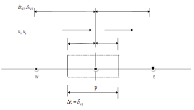
The finite volume method is a method for representing and evaluating partial differential equations in the form of algebraic equations[3]. Similar to the finite difference method or finite element method, values are calculated at discrete places on a meshed geometry. "Finite volume" refers to the small volume surrounding each node point on a mesh. In the finite volume method, volume integrals in a partial differential equation that contain a divergence term are converted to surface integrals, using the divergence theorem. These terms are then evaluated as fluxes at the surfaces of each finite volume. Because the flux entering a given volume is identical to that leaving the adjacent volume, these methods are conservative. Another advantage of the finite volume method is that it is easily formulated to allow for unstructured meshes. The method is used in many computational fluid dynamics packages. In finite difference,[5] the dependent variable values are stored at the nodes only. Infinite element method, the dependent values are stored at the element nodes. But in finite volume method, the dependent values are stored in the centre of the finite volume. In FVM, conservation of mass, momentum, energy is ensured at each cell/finite volume level. This is not true in finite difference and finite element approach. It is always better to use governing equation in conservative form with finite volume approach to solve any problem which ensures conservation of all the properties in each cells/control volume. One advantage of the finite volume method over finite difference methods is that it does not require a structured mesh (although a structured mesh can also be used).Now we shall discuss the steps involving FVM for solving differential equation:Step 1: Grid GenerationThe first step in the finite volume method is grid generation by dividing the domain in to discrete control volumes. Let us place a number of nodal points in the space between A and B. The boundaries of control volumes are positioned mid-way between adjacent nodes. Thus each node is surrounded by a control volume or cell. It is common practice to set up control volumes near the edge of the domain in such a way that the physical boundaries coincide with the control volume boundaries. A general nodal point defined by and its neighbours in a one-dimensional geometry, the nodes to the west and east, are defined by W and E, respectively. The west face of the control volume is referred by ‘w’ and east side by ’e’. The distances of these points are given in figure.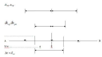 Step 2: DiscretizationThe most important features of finite volume method are the integration of the governing equation over a control volume to yield a discretized equation to yield a discretized equation at its nodal points P.Step 3: SolutionAfter discretization over each volume method, we are finding a system of algebraic equation. Which are easily solved by numerical scheme such as Gauss-Siedel method. Generally equations are in tri-diagonal form in next section we are describing this method by a suitable example
3. Finite Volume Method for Real Life Problem
In this section, we describe the finite volume method for solving convection-diffusion problem. Firstly, we shall define a convection-diffusion problem.Convection-diffusion problemThe general transport equation for any fluid property is given by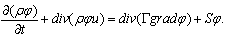 | (1) |
In problems where fluid flow plays a significant role we must account for the effects of convection. Diffusion always occurs alongside convection in nature so here we examine method to predict combined convection and Diffusion. The steady convection-diffusion equation can be derived from transport equation (1) for a general property by deleting transient term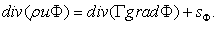 | (2) |
Formal integration over control volume gives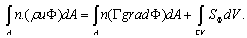
 In the absence of sources, the steady convection and diffusion of a property in a given one-dimensional flow field u is governed by
 | (3) |
And continuity equation becomes  Integrating equation (3) and we have
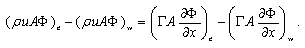 And continuity equation becomes
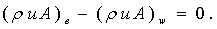 To obtain discretized equation, we shall take some assumption:Let
  represent convective mass flux per unit area and
  represent diffusion conductance.Now we are taking
  and applying the central differencing the integrated convection-Diffusion becomes
 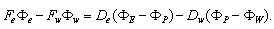 | (4) |
And continuity equation becomes | (5) |
Central differencing schemeThe central differencing approximation has been used to represent the diffusion terms which appears in equation (4).So Putting these values on equation (4) becomes
 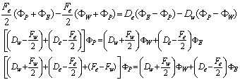 | (6) |
Equation (6) can be written as  | (7) |
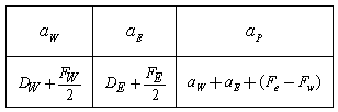
Where 
 and
and  are coefficients of
 and
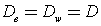
and  respectively. Example: A property
  is transported by means of convection and diffusion through the one dimensional Domain the governing the governing equation is given below boundary conditions are
 at x=0 and
  at x=L. using five equally spaced cells and the central differencing scheme for convection and diffusion calculate the distribution of
  as a function of x for Case (1): u=0.1 m/sCase (2): u=2.5 m/sThe following data apply
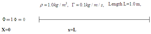 SolutionIt is given that u=0.1 m/s let domain is divided in to five control volume so
  m. Let
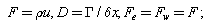
 everywhere. The boundaries are denoted by A and B.
 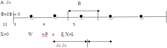 The discretization of equation (7) and its coefficient apply at internal nodal points 2, 3, 4, but control volume 1 and 5 need special treatment we integrate equation (3) and using central differencing for both diffusion and convective flux through the east face of cell 1.
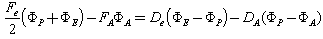 | (8) |
and similarly for control volume 5, we may write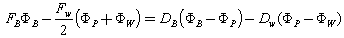 | (9) |
But value of  in west face and east face is given
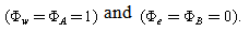 | (10) |
Using (10) in equation (8) and (9) and rearranging, we note that and
and gives discretized equation at boundary nodes of the following form
  | (11) |
and central coefficients are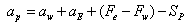 | (12) |
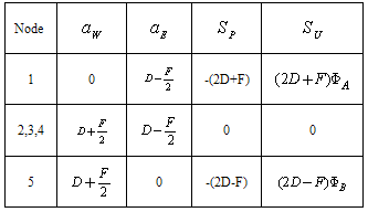 Case1:
  gives the coefficient as summarized as given below
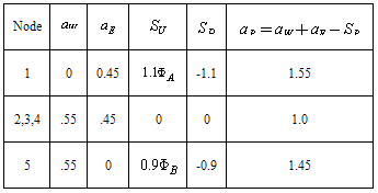
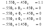 The algebraic equations are given below
 The solutions of above equations are given below:
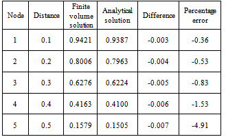 Case (2): In this case velocity is u=2.5 m/s, flow term is.
  . Thus coefficients are given below:
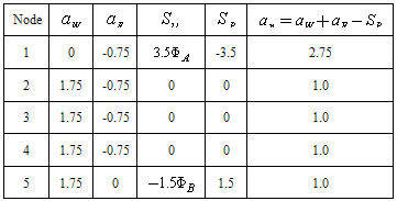 The discretizing equations are given below
  The matrix form is
  Solution of the problems is
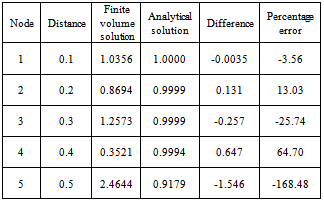 After solving this problem, we see that, when velocity is u=0.1, then numerical solution converges to analytical solution but when u = 2.5 then solution for final grid node diverges, but when we are taking 20 grid nodes then numerical solution converges this is due to velocity 25 times more than u = 2.5 this problem occur very frequently in convection-diffusion problems. It happen when velocity is large then convection is dominated and velocity is small then diffusion is dominated to omit these problems. There are two methods, first is that increase grid size and second one is that set up new scheme, known as up-winding but this differencing scheme is not focus of our paper.
4. Finite Difference Method
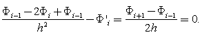
S. M. Choo et.al. published an article[8] “High-order perturbation-difference scheme for a convection diffusion problem” using finite difference methods and with uniform meshes considered for a one-dimensional singularly perturbed convection diffusion problem. In order to obtain high-order of convergence, the difference methods are combined with a perturbation technique. The methods have uniform convergence and did not give non-physical oscillations in the numerical solutions. Existence and corresponding error estimates of the solution for the difference schemes have been shown. Numerical experiments were provided to back up the analysis.In mathematics and engineering, finite-difference methods[6] are numerical methods for approximating the solutions to differential equations using finite difference equations to approximate derivatives (11). Assuming the function whose derivatives are to be approximated is properly-behaved, by Taylor's theorem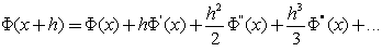 | (13) |
From which we obtain 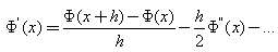 Thus, we have
  | (14) |
Which is the forward difference approximation for . Similarly expansion of
  in Taylor’s series gives.
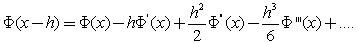 | (15) |
From which we obtain | (16) |
which is the backward difference approximation for .Subtracting equation (15) from equation (!3) we obtain the following central difference approximation:
 | (17) |
It is clear that central difference approximation is better than backward and forward difference approximation. Similarly, we can obtain approximation for higher order derivative terms, such as adding equations (13) and (15), we get .
. | (18) |
To solve given boundary value problems, we can divide the range  in to n equal subintervals of width h so that
  i=1,2, ,n.The corresponding value of
  at these points are denoted by
  Thus from equation (17) And (18) we obtain
 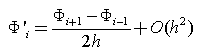 and
and 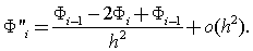 We solve the above problem by finite difference method for same nodal points and finding how FVM is better than Finite difference method.Case1: U=0.1Since the governing equation is
  , we can write this equation in discretized form as for
 After simplifying this equation we may write
  Thus set of algebraic equation is
  In matrix form the above set of algebraic equations may be written as
 After solving above equation, we have
 Case2: U=2.5In this case, the discretized equation is
  The above equation may be written in matrix form as:
 The solution of above system of equation is given below:
 Result:The result and graph of both cases are given below.Case1: U=0.1
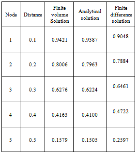
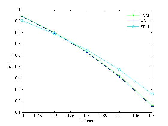 | Figure 1. Comparison of FVM and FDM with Analytical Solution (AS), U=0.1 |
Case2:U=2.5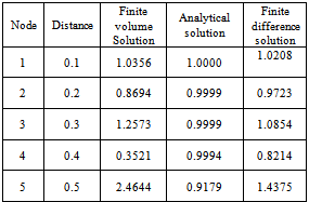
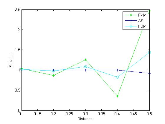 | Figure 2. Comparison of FVM and FDM with Analytical Solution (AS), U=2.5 |
5. Conclusions
After analysing the results and by above discussion, we see that when velocity is larger, finite volume solution does not have better convergence. The reasons for this are given below:1. The internal coefficients of discretized scalar transport equation (7) are A steady one-dimensional flow field is also governed by the discretized continuity equation (5).When this equation holds then flow field satisfies continuity and also satisfiesScarborough condition, which is given as  2. In case two when velocity is 2.5 m/s, the solution does not provide better convergence, with
 The convective contribution to the east coefficient is negative; if the convection dominates it is possible for to be negative. Given that
  and
and  (that is flow is unidirectional), for
  to be positive
  and
and  must satisfy the condition
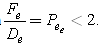 If
If is greater than two then east confidents will be negative. This violates one of the requirements for boundedness and may lead to physically impossible solution. These types of problems are called convection-dominated problems. It is well known that the convection-dominated diffusion problem has strongly hyperbolic nature; the solution often develops sharp fronts that are nearly shocks. So the finite difference method or finite element method does not work well when problem is convection dominated[13].
References
| [1] | B. Guo and X. Wang, Testing of new high-order finite difference methods for solving the convection-diffusion equation, E-Journal of Reservoir Engineering, 1,(1)(2005), 1-14 |
| [2] | C. Japhet, F. Natafand and F. Rogier, The optimized order two method Application to convection-diffusion problems, Future Generation Computer Systems, 18(1)(2001), 17-30 |
| [3] | J. D. Anderson, Computational Fluid Dynamics: The Basics with Applications, Macgraw-Hill Publications, Edition 6, 2008. |
| [4] | H. Versteeg and W. Malalasekra,, An Introduction to Computational Fluid Dynamics: The Finite Volume Method, Lomgman Scientific and Technical Publishers, 1995. |
| [5] | Tapan K Sengupta and Orient Longman, Fundamentals of Computational Fluid Dynamics, Orient Longman Pvt. Ltd., 2004. |
| [6] | P. K. Kundu and I. M. Cohen, Mechanics, third edition, Elsevier, 2004. |
| [7] | Randall J. Leveque, Finite Volume Methods for Hyperbolic Problems, Cambridge University Press, 2002. |
| [8] | S.M. Choo and S.K. Chung, High-order perturbation-deference scheme for a convection diffusion problem, Computer Methods in Applied Mechanics and Engineering, 190(10)(2000), 721-732. |
| [9] | F. Nataf, F. Rogier and E. de Sturlerin: A. Sequeira (Ed.), Navier–Stokes Equations on Related Nonlinear Analysis, Plenum Press, New York, 1995, 307–377. |
| [10] | Y. Saad, Iterative Methods for Sparse Linear Systems, PWS Publishing Company, 1996. |
| [11] | B. Garcia-Archilla and J. A. Mackenzie, Analysis of a super convergent cell vertex volume method for one-dimensional convection-diffusion problems, IMA Journal of Numerical Analysis, 15(1995), 101-115. |
| [12] | C. Japhet, Méthode de decomposition de domaine et conditions aux limitesartificielles en mecanique des fluides: method optimised’Ordre 2, Thèse de Doctorat, Université Paris XIII, 1998; F. Nataf, F. Rogier, M3 AS, 5 (1) (1995) 67–93. |
| [13] | L. Quian, X. Feng and Y. He, The characteristic finite difference streamline diffusion method for convection-dominated diffusion problem, Applied Mathematical Modeling, 36 (2012), 561-572. |
 Abstract
 Reference
 Full-Text PDF
 Full-text HTML