1. Introduction

SFS deals with the recovery of surface orientation and surface shape (highlight) from the gradual variation of shading in images. SFS is implemented by first modeling the image brightness as a function of surface geometry and then reconstructing a surface which, under the given imaging model, generates an image close to the input image. This field was formally introduced by Horn[1] and there have been many significant improvements in both theoretical and practical aspects of the problem.

However, it has been shown that this is an ill-posed problem[2,3]. Surface shape recovery of observed objects is one of the main goals in the field of three-dimensional (3-D) computer vision. Marr identified shape-from shading (SFS) as providing one of the key routes to understanding 3D surface structure via the 2½D sketch[4]. The process has been an active area of research for over two decades. It is concerned with recovering 3D surface shape from shading patterns. The subject has been tackled in a variety of ways since the pioneering work of Horn[5].

They are classified into direct and indirect methods. Direct or active methods recover depth information directly using range finder and structure light. Indirect methods determine the relative depth by cues extracted from gray level images of observed object. This class contains shape from shading. Since the direct or active techniques usually involvemany complex external component setup, they may not be suitable for instance in object shape estimation. Hence many researchers have focused on the latter class of method. The shape from shading methods makes use of the change in image brightness of an object to determine the relative surface depth and can be effectively applied to smooth surface regions. Most of the shading techniques employ variation approaches which impose constraints such as smoothness, imaging equation and light conditions.

As a result these techniques can only be applied to the object surface that satisfies the constraints. Also the computational complexity of the resulting algorithms is high and increases as the number of these constraints increases. Useful alternatives for variation shading are local shading and linear shading suggested by Pentland[6] this approach do not require prior information on the observed scene, imaging geometry and regularization. The assumption is that the surface shape is locally spherical, and the inclined light source is not allowed. Pentland[7] used the linear approximation of the reflectance function in terms of the surface gradient and applied a Fourier transform to the linear function to get a closed form solution for the depth at each point. Tsai and Shah[8] applied the discrete approximation of the gradient first, then employed the linear approximation of the reflectance function in terms of the depth directly. Their algorithm recovered the depth at each point using a Jacobi iterative scheme. As opposed to the previous methods on SFS, Samaras and Metaxas[9] presented a model-based approach, where shape from shading is incorporated as a nonlinear hard constraint within a deformable model framework. Recently, Zhao and Chellappa[10] provided a shape from shading approach for symmetric objects. A recent minimization based method proposed in[11] directly solves the shape by assuming the depth of the deepest surface point is known under constant albedo approximation. Alper and Mubarak[12] proposed a shape from shading (SFS) approach to recover both the shape and the reflectance properties of symmetric objects using a single image. The common constraint of constant or piece-wise constant albedo for Lambertian surfaces is relaxed to arbitrary albedo. The proposed method can be categorized as a linear shape from shading method, which linearizes the reflectance function for symmetric objects using the symmetry cues of the shape and the albedo, and iteratively computes the depth values. Estimated depth values are then used to recover pixel-wise surface albedo.

In this study, the GA is applied to 3-D shape reconstruction of an object from a shading image of the object. In this method, arbitrary 3-D shapes are defined as individuals in a population according to the GA concept. The evaluation function of each individual is defined according to the correspondence between the 3-D shape represented by the individual and the measured 2-D shading image and other information about the object's 3-D shape, and then the optimized solution of the function is searched for using a GA. Accordingly, the 3-D shape represented by the individual having the highest value of the evaluation function is considered as the reconstructed 3-D shape of the object. The principle of the proposed method for reconstructing a 3-D shape from a 2-D shading image using a GA is described. For demonstration of the proposed method, 3-D shapes are reconstructed from shading images which are obtained by both computer simulation and experiment with a CCD camera. The reconstructed shapes are compared with shapes reconstructed by the conventional method of obtaining a shape from shading[13].

2. Related Works

There are two ways to recover shape from a single image namely shape from shading and user interactive modeling [14]. The non-interactive methods compute depth based on the work proposed by Horn and Brook. This is done by minimizing the Eikonal equation and presenting the solution as computed depth. In the interactive method, the depth map obtained is interactively modified by the user in order to get more accurate results. Zhang et al.[15] classified shape from shading methods into four groups viz. minimization, propagation, local and linear methods. Zhang et al. implemented 6-well known algorithms and compared them objectively based on COP time and error. Although each algorithm works well with specific image, but produces poor results with others. In another work Durou et al.[16] classified shape from shading methods into three classes: minimization approaches, approximation approaches and partial differential equation based approaches.

Patel and Smith[17] used a morphable model for shape from shading of non-Lambertian surfaces. Shlizerman and Basri[18] used the similarity between faces for 3D reconstruction. Common face features such as location of eyes, aspect ratio and the location of nose can vary between different races, gender or because of facial expressions. Using previously stored features their proposed algorithm guides the reconstruction of the face using information about the subject race, gender and facial expressions.

3. Problem Formulation

We start by giving a brief outline of the SFS problem and introducing the basic assumptions. We attach to the camera a three-dimensional coordinate system (Oxyz), such that Oxy coincides with the image plane and Oz coincides with the optical axis. Under the assumption of orthographic projection, the visible part of the scene is, up to a scale factor, a graph z = u(x), where x = (x,y) is an image point. As is well known[19], the SFS problem can be modeled by the "image irradiance equation":

(1)

where I(x) is the greylevel measured in the image at point x (in fact, I(x) is the irradiance at point x, but both quantities are proportional) and R(n(x)) is the reflectance function, giving the value of the light re-emitted by the surface as a function of its orientation, i.e. of the unit normal n(x) to the surface at point (x,u(x)). This normal can easily be expressed as:

(2)

where p= d and q =, so that u(x) = (p(x), q(x)). Irradiance function I is the datum in the model since it is measured at each pixel of the image, for example in terms of a greylevel (from 0 to 255). To construct a continuous model, we will assume that I takes real values in the interval[0,1]. Height function u, which is the unknown of the problem, has to be reconstructed on a compact domain ², called the ‘‘reconstruction domain’’. Assume that there is a unique light source at infinity whose direction is indicated by the unit vector ³. Also assume for simplicity that x is given (in some works, x as well is considered as unknown, see e.g.[20,21], even if this new problem is sometimes ill-posed[22]). Recalling that, for a Lambertian surface of uniform albedo equal to 1, R(n(x)) = n(x), Eq.1 can be written, using Eq.2:

(3)

which is a first order non-linear partial differential equation (PDE) of the Hamilton–Jacobi type. Points such that I(x) is maximal correspond to the particular situation where x and n(x) point in the same direction: these points are usually called ‘‘singular points’’. Let us mention that Eq. (3) is not the most general equation of SFS[23]: since real materials are not purely Lambertian, some publications are concerned with non-Lambertian SFS problems [24–26]; moreover, the situation is more complex in the presence of other lighting models[27,28] or when the interreflections are taken into account[29,30]. We will also consider the equation which appears in most of the papers and corresponds to frontal light source at infinity, i.e. . Then Eq.3 becomes the "eikonal equation":

(4)

(5)

Equations 3 or 4 are sometimes complemented with boundary conditions on ∂Ω or with additional information to select a unique solution. One can set up a boundary value problem which imposes either a value to the solution u (Dirichlet type boundary condition), or a value on the normal derivative (Neumann type boundary condition), or a so-called ‘‘state constraint’’ boundary condition where one imposes an equation to be satisfied on the boundary. For an image containing an ‘‘occluding boundary’’, it is usual to use it as boundary ∂Ω of the reconstruction domain Ω. For example, in Figure. 1, if the part of the image representing the object in greylevels (‘‘silhouette’’) is Ω, then ∂Ω coincides with the occluding boundary. A current choice is to consider Dirichlet type boundary conditions in order to take into account (at least) two different possibilities. The first corresponds to the assumption that the surface is standing on a flat background, i.e. we set:

(6)

The solution of Eq. 3 or of the Dirichlet problems 3-6 will give the surface corresponding to greylevel I(x) measured in Ω.

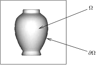Figure 1. Object with occluding boundary, which might be used as boundary

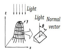Figure 2. The normal vector of the surface and the direction of the light source.

4. Shape From Shading Using GA

4.1. Shading Images

Gray levels in a shading image are determined by the orientation of the object surface. Assuming that the surface of the object is Lambertian, the gray levels of the shading image are expressed as the following Eq.7.

(7)

where represents surface reflectance constant, and is the angle between the normal vector of the surface and the direction of the light source as shown in Figure. 2. In other words, a shading image of an 3-D object provides some information on the surface orientation of the object. However, the orientation cannot be uniquely determined. Therefore some constraint on the shape of the object is required for 3-D shape reconstruction from a shading image.

4.2. Reconstruction Using GA

In our proposed method, we assume that the constraints on the 3-D shape of an object are follows: (a) the boundary of the object in the shading image is specified, (b) the object does not have hollows and (c) the surface of the object is smooth.

To apply a GA based matrix code , the candidates to be optimized must be coded as strings. In this method, a 3-D shape of the object is represented by a 2-D range image of L x L pixels with M levels, and then the range image is a coded string. Here, the pixels outside of the object boundary are set to zero according the condition (a). Figure. 3 shows the method for coding a 3-D shape. According to the coding method, the optimized 3-D shape is searched for using a GA as follows:

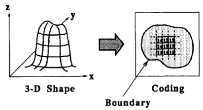Figure 3. The method for coding a 3-D shape. The string representing a 3-D shape is a range image of L x L pixels with M levels.

Firstly, make a initial population of N strings. When a 3-D shape is represented by the string as described above, the total number of candidates of 3-D shapes is very large, i.e. where is the number of pixels inside the boundary of the object. accordingly, it becomes very difficult to find the optimal 3-D shape because the area to be searched is very wide. Hence, 3-D shapes represented by strings are restricted according to the condition (b), so that the total number of candidates of 3-D shapes can be reduced, and the efficiency of an optimal search can be improved. In making the initial population, strings are produced by matrix code.

This method starts with an initial population P₀ of size μ. This initial population is coded as a matrix of size μ× n called initial population matrix PM₀. At every generation t, PM_t is partitioned into v × η sub- matrices i = 1..., v, j = 1..., η, where v is the number of individuals on each partition and η is the number of genes on each partition.

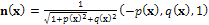
A crossover and mutation operators are applied on the partitioned sub-matrices and is updated. The range of each gene is divided into m sub-ranges in order to check the diversity of the gene values. The Gene Matrix GM is initialized to be the n × m zero matrix in which each entry of the i-th row refers to a sub-range of the i-th gene. While the search is processing, the entries of GM are updated if new values for a gene are generated within the corresponding sub-range. After having a GM full, i.e., with no zero entry, the search is learned that an advanced exploration process has been achieved. The Gene Matrix GM comes along with a certain number α predefined by the user. The zeros entries in GM are not immediately updated to be ones unless the number of individuals that have been generated inside a sub-range so far exceeds or equals αm.

An example of GM with α = 0.2 in two dimensions is shown found in Figure. 4. In this figure the range of each gene is divided into ten sub-ranges. We can see that no individual has been generated inside the sub-ranges 1, 7 and 10 for the gene x₁. However entry (1, 3) in GM0.2 is equal to 0 since there is only one individual lying inside the third sub-range and αm = 2. For the same reason, x₂ has six zero-entries corresponding to six sub-ranges in which the number of generated individuals is less than αm. In a succeeding generation, if one or more individuals are generated inside the third sub-range for x₁ for example, then entry (1, 3) will be set equal to one. In our experiments we used α as a function of log(n) and log(μ), where μ is the population size, in order to be suitable for all dimensions and for all population size. Moreover, the log function is used to estimate the value of α in order to reduce the complexity of increasing n or μ especially in high dimensional problems. Actually, the numerical experiments have showed that the best setting for number α is equal to 0.75 log² n log μ. And then we calculate a fitness function for each string. Each string represents a 3-D shape that can determine a 2-D shading image. The fitness value of the string is defined according to the similarity the shading image determined by the string with the measured shading image. The fitness value is expressed as the following Eq.8:

(8)

where

C= a constant for making the fitness positive.

= a shading image determined by a string which is a candidate of the object shape,

= smoothing image of S ( i , j ) ,

= the measured shading image,

A smoothing image of is expressed as

(9)

A shading image determined by a string is calculated according to equation (9). In the definition of the string fitness, a smoothing image of it shading image determined by a string is compared with the measured shading image. We consider this to mean that condition (c) is true.

Secondary, arithmetical crossover and mutation operations are used in the proposed algorithm to crossover operation between individuals from the current population into next generation. We can defined in the following procedure.

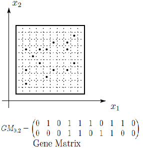Figure 4. An Example of the Gene Matrix in .

Procedure Crossover (p¹, p²)

Choose randomly a number α from (0,1)

Two offspring and are generated from parents and where

1- Return.

The proposed method uses mutation operator by generating a new random value for the selected gene within its domain. Mutagenesis. In order to accelerate the search process, a special type of a directed mutation is applied. Actually, our method employs the mutagenesis operator [31]. Mutagenesis is used to alter some individuals selected for the next generation. The formal procedure for mutagenesis is given as follows.

Procedure 2. Mutation(x,GM)

1. If GM is full, then return; otherwise, go to Step 2.

2. Choose a zero-position (i, j) in GM randomly.

3. Update x by setting ,

where r is a random number from (0, 1)

and l_i, u_i are the lower and upper bounds of the variable , respectively.

4. Update GM and return.

The algorithm described as follows.

Initialization Set values of m, μ, v and η . Set the crossover and mutation probabilities pc (0,1) and pm (0,1), respectively. Set the generation counter t := 0. Initialize GM as n × m zero matrix, and generate an initial population P₀ of size μ and code it to a matrix

Parent selection. Evaluate the fitness function of all individuals coded in Select an intermediate population from the current one .

3- Partitioning and genetic operations. Partition into v × η sub-matrices. Apply the following for all sub-matrices , i = 1..., η, j = 1..., v.

3.1. Crossover. Associate a random number from (0, 1) with each row in and add this individual to the parent pool if the associated number is less than pc. Apply Procedure crossover to all selected pairs of parents and update

3.2. Mutation. Associate a random number from (0, 1) with each gene in each gene i

. Mutate the gene which their associated number less than pm by generating a new random value for the selected gene within its domain.

4- Stopping condition. If GM is full, then go to Step 7. Otherwise, go to Step 5.

5-Survivor selection. Evaluate the fitness function of all corresponding children in , and choose the μ best individuals from the parent and children populations to form the next generation .

6- Mutagenesis. Apply procedure 2 to alter the worst individuals in , set t:=t+1 and go to Step 2.

7-Intensification. Apply a local search method starting from each solution from the N_elite elite ones obtained in the previous search stage.

5. Experimental

It is very difficult to choose good test images for SFS algorithms. A good test image must match the assumptions of the algorithms, e.g. Lambertian reflectance model, constant albedo value, and infinite point source illumination. It is not difficult to satisfy these assumptions for synthetic images, but no real scene perfectly satisfies these conditions. In real images there will be errors to the extent that these assumptions are not matched. In this section, we describe the images chosen to test the SFS algorithms.

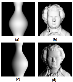Figure 5. Synthetic images generated using two different light sources: (a) Synthetic Vase (0, 0, 1), (b) Mozart (0, 0, 1), (c) Synthetic Vase (1, 0, 1) and (d) Mozart (1, 0, 1).

The synthetic images were generated using true depth maps, we simply computed the surface gradient where p= and q = using the forward discrete approximation of the depth, u and generated shaded images using the Lambertian reflectance model. There are at least two advantages of using synthetic images. First, we can generate shaded images with different light source directions for the same surface. Second, with the true depth information, we can compute the error and compare the performance. However, the disadvantage of using synthetic images is that performance on synthetic images cannot be used reliably to predict performance on real images. In our study we used two synthetic surfaces (Synthetic Vase and, Mozart), with two different light sources ((0, 0, 1) and (1, 0, 1)). Also in our study we used three real images (Lenna, Pepper and Vase), shown in Figures. 5 and 6. The light source directions for these images are the following: for the Lenna image light source direction is (1.5, 0.866, 1). And Pepper image light source direction is (0.766, 0.642, 1), finally Vase image is (-0.939, 1.867, 1.0).

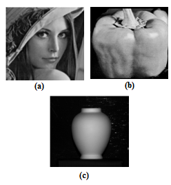Figure 6. Real images: (a) Lenna. (b) Pepper. (c) Vase

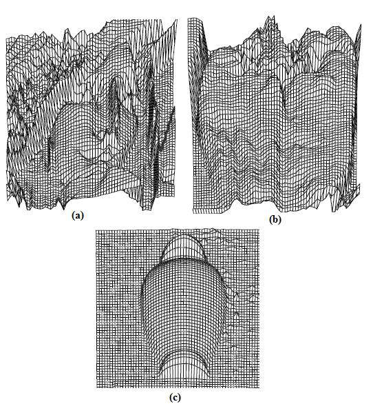
Figure 7. Results for Zheng and Chellappa's method on synthetic images: (a) Vase, (b) Mozart, (a) and (b) show the results for test images with light source (0, 0, 1). (c) and (d) show the results for test images with light source (1, 0, 1).

In order to prove the efficiency and accuracy of our approach, we used synthetic and real world images as test data sets. Among them, one synthetic image was used to verify whether the proposed approach is accurate. On the other hand, three real images were used to examine how well this method works. All test images were of size . Table 1 summarizes the parameters of each image

Table 1. The parameters of used image Image Mozart 0.0 0.0 1.0 0.51 0.050 Pepper 0.5 0.5 1.5 0.40 0.010 Vase 0.5 0.5 -1.0 0.70 0.005 Lenna 1.5 0.8 1.0 0.50 0.050

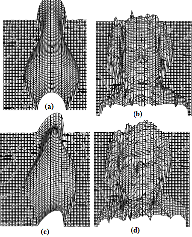Figure 8. Results for Tsai and Shah's method on synthetic images: (a) Vase, (b) Mozart(a), and (b) show the results for test images with light source (0, 0, 1). (c) and (d) show the results for test images with light source (1, 0, 1).

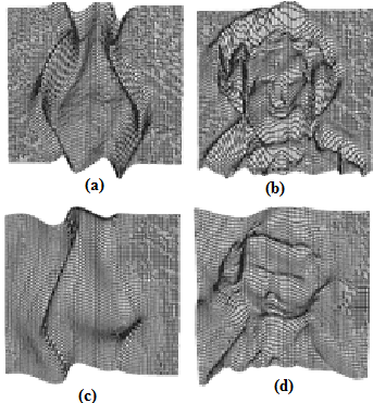
Figure 9. Results for Zheng and Chellappa's method on real images: (a) Lenna. (b) Pepper. (c) Vase

Figure 10. Results for Tsai and Shah's method on real images: (a) Lenna. (b) Pepper. (c) Vase.

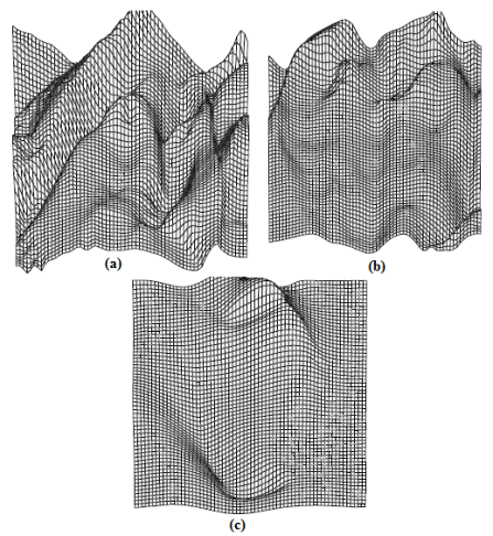
The parameters , , and were estimated by Zheng and Chellappa method. The parameter is always positive, and was determined experimentally. Figure. (11) shows the experimental results of a synthetic Mozart image. Figure (11.a) shows the original image. The surface recovered by our approach is shown in Figure (11.b). In order to verify the accuracy of the proposed approach, it was necessary to apply our algorithm on natural images. The next examples show the results obtained by applying our approach to the Pepper ,Vase, and Lenna. The recovered surface is shown in Figures (12, 13 and 14). For the reconstructed pepper image in Figure (13), there is some errors due to albedo discontinuities and self-occlusions, which violate the assumptions of the algorithm[32]. The effect of different GA parameters on the reconstruction accuracy is investigated. The GA parameters used in the algorithm are summarized in Table 2.

Table 2. The GA parameters Parameters Definitions Values Population size 25 η No. of gene partitions n/5 v No. of individual partitions 5 α Gene matrix percentage 0.75 log2 n log μ Pc Crossover probability 0.7 Pm Mutation probability 0.002 m No. of GM column Nmax No. of maximum iterations 5n Nelite No. of best solution for intensification 1

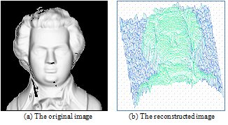Figure 11. Results for our method on synthetic image “Mozart”.

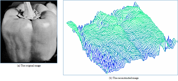Figure 12. Results for our method on real image “Pepper”.

In order to assess the proposed approach with the other existing approaches of SFS, Table 3 demonstrates a comparison between the proposed approach and existing approaches. Further, Table 3 shows that the proposed approach has achieved acceptable degree of success with less processing time compared to existing approaches.

Table 3. C.P.U. time (in seconds) for synthetic images. Method Images Vase Mozart S1 S2 S1 S2 Zheng & Chellappa 18.1 70.8 49.6 409.5 Tsai & Shah 0.9 1.2 3.8 4.8 Proposed method 0.1 0.55 1.06 1.56

(Note: S₁ and S₂ stand for two different light sources, (0, 0, 1) and (1, 0, 1)).

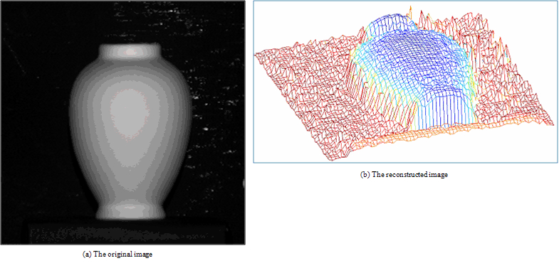Figure 13. Results for our method on real image “Vase”

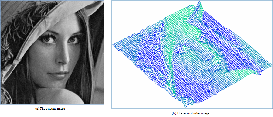Figure 14. Results for our method on real image “Lenna”

6. Conclusions

In this paper, a new method for solving the Shape from Shading problem using GA based on matrix code has been developed. The novelty of the proposed technique comes from the GA itself. This has been achieved by applying an efficient multi objective function with the brightness and smoothness constrains. Several GA design parameters have been studied to illustrate their effects on the algorithm convergence. The proposed method is tested in both synthetic and real image and is found to perform accurate and efficient results as shown in Table 3.