H. Naroua 1, A. S. Sambo 2, P. C. Ram 3
1Département de Mathématiques et Informatique, Université Abdou Moumouni, B.P.10662, Niamey, Niger
2Energy Commission of Nigeria, Plot 701c, Central Area, Opposite National Mosque, PMB 258, Garki-Abuja, Nigeria
3Department of Mathematics and Computer Science, The Catholic University of Eastern Africa, P. O. Box 62157, Nairobi, Kenya
Correspondence to: H. Naroua , Département de Mathématiques et Informatique, Université Abdou Moumouni, B.P.10662, Niamey, Niger.
| Email: |  |
Copyright © 2012 Scientific & Academic Publishing. All Rights Reserved.
Abstract
In this paper, the finite element method is employed in order to study the MHD free convection heat generating fluid flow past an impulsively started vertical infinite plate when a strong magnetic field is imposed in a plane which makes an angle α with the normal to the plate. Numerical calculations have been carried out on the velocity and temperature distributions which are depicted graphically. The results obtained are discussed extensively in terms of the different parameters entering into the problem.
Keywords:
Computer Program, Finite Element Method, Hall Currents, Modeling, MHD
Cite this paper:
H. Naroua , A. S. Sambo , P. C. Ram , "A Computational Solution of MHD Stokes Problem for a Heat Generating Fluid with Hall Currents", American Journal of Computational and Applied Mathematics , Vol. 1 No. 1, 2011, pp. 1-5. doi: 10.5923/j.ajcam.20110101.01.
1. Introduction
In recent years, considerable interest has been given to the theory of rotating fluids due to its application in cosmic and geophysical sciences. In an ionized gas where the density is low and/or the magnetic field is very strong, the conductivity normal to the magnetic field is reduced due to the free spiraling of electrons and ions about the magnetic lines of force before suffering collisions and a current is induced in a direction normal to both the electric and magnetic fields. The effect of Hall currents on the Stokes problem has provided a new dimension in its application to MHD power generators and extended problem of ionized plasma flow in the presence of special configuration of magnetic field. One of the most important applications of this problem is in the study of coronal plasma flow in the configuration of plasma sheet formation in the active region of the sun or in the magnetic tail region. The Stokes problem under transversely applied magnetic field was studied by Rossow[1] whereas the corresponding MHD problem for a vertical impulsively started infinite plate was studied by Soundalgekar et al[2]. When the gas or fluid is partially ionized, the Hall current becomes significant and plays an important role in the development of the flow field. Although many improvements have been made in tackling this problem, we have chosen a computational solution based on the finite element analysis. Pop[3] studied the effect of Hall currents on hydromagnetic flow near an accelerated plate when the magnetic field is imposed normal to the plant. The problem of Hall current has alsobeen considered by a number of authors[4-7]. It is now proposed to study, by the finite element method, the MHD free convection of a heat generating fluid flow past an impulsively started vertical plate taking into account the Hall currents when a strong magnetic field is imposed in a plane which makes an angle α with the normal to the plate.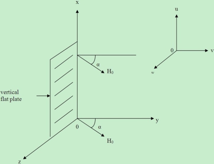 | Figure 1. The flow configuration with the coordinate system used. |
2. Mathematical Analysis
Consider the MHD free-convection heat generating fluid flow past an infinite vertical plate started impulsively in its own plane. The x/-axis is taken along the plate in the vertically upward direction and the y/-axis is taken normal to the plate. Initially, the temperatures of the plate and the fluid are assumed to be the same. At time t/>0, the plate starts moving impulsively in its own plane with velocity U0 and its temperature is instantaneously raised or lowered to which is maintained at a constant value. The fluid is permeated by a strong magnetic field H = (0, λH0,  ), where λ = cosα, α being the angle made by H with the normal to the plate. The flow configuration, together with the coordinate system used, is shown in Figure1. Since the plate is infinite in length, all variables are functions of y/ and t/ only. It is assumed that the induced magnetic field is negligible. This assumption is justified when the magnetic Reynolds number is very small (Shercliff,[8]).The equation of conservation of electric charge
  gives
gives  = constant where
 . This constant is zero since
  = 0 at the plate, which is electrically non-conducting. Thus,
  = 0 everywhere in the flow.Next, we consider the case of a short circuit problem in which the applied electrical field E = 0. When the strength of the magnetic field is very large, the generalized Ohm’s law in the absence of an electric field (Cowling,[9]) is given by:
 | (1) |
where σ, μe, ωe, τe, e, ne, Pe and Q are defined in nomenclature. Neglecting the electron pressure, the thermoelectric pressure and the ion slip, we have: | (2) |
 | (3) |
where m = ωeτe is the Hall parameter.By applying the usual boundary layer approximation, the flow is governed by the following equations: | (4) |
 | (5) |
 | (6) |
In equations (4)-(6), the inertia terms are neglected as we are considering only fully developed flow. Hence, our results are true for short times after the motion and temperature jump at the wall.The initial boundary conditions of the problem are given by:t/ ≤ 0: u/ = 0, w/ = 0, T/ =  everywhere
 | (7) |
We now introduce the following non-dimensional quantities as defined in the nomenclature: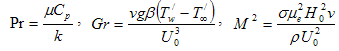 | (8) |
Using the above formulation, equations (4) – (6) reduce to :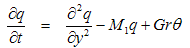 | (9) |
 | (10) |
Where q = u+iw and  denotes the complex conjugate of q.The corresponding boundary conditions are:
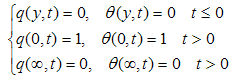 | (11) |
For simplicity in the calculations, we consider m=0 and λ=1 which reduce M1 to a real number M2. In view of this, Equations (9) and (10) can be rewritten as: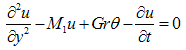 | (12) |
 | (13) |
 | (14) |
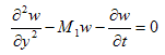
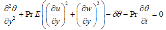
The above system of Equations (12 - 14) with boundary conditions (11) has been solved numerically by a computer program using the finite element method in steps 1, 2 and 3.Step 1: We solve Equation (14) with the help of boundary conditions (11). Constructing the quasi - variational equivalent of Equation (14), we have: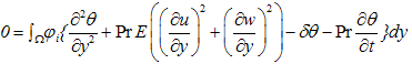 | (15) |
where  denotes the test function and is the domain of the flow.Consider an N elements mesh and a two parameter (semi discrete) Galerkin approximation[10,11] of the form:
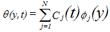 | (16) |
with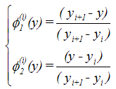 | (17) |
where i = 1,2,3,…,N and yi and yi+1 are respectively the lower and upper coordinates of the element i. Using Equations (16 - 17), Equation (15) reduces to: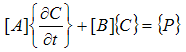 | (18) |
where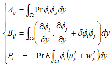 | (19) |
Using the Θ - family of approximation developed by Reddy [11], Equation (18) reduces to: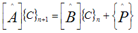 | (20) |
where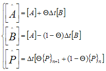 | (21) |
The initial value C0 is obtained by the Galerkin method from a 32 elements mesh and is given by: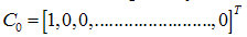 | (22) |
For t > 0,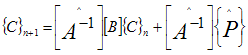 | (23) |
Step 2: We solve Equation (12) with the help of boundary conditions (11). Constructing the quasi - variational statement of Equation (12), we have: 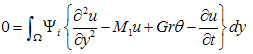 | (24) |
where Ψi is the test function and Ω is the region of the flow.Consider a two parameter (semi-discrete) Galerkin approximation[10,11] of the form: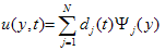 | (25) |
with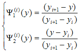 | (26) |
where i=1,2,3,…..,N and yi and yi+1 are respectively the lower and upper coordinates of the element i.Using Equations (25-26), Equation (24) reduces to: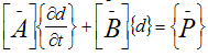 | (27) |
where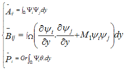 | (28) |
Using the Θ - family of operators developed by Reddy [11], Equation (27) takes the form: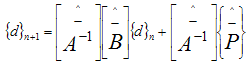 | (29) |
where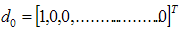 | (30) |
Step 3: We solve Equation (13) with the help of boundary conditions (11). Constructing the quasi - variational statement of Equation (13), we have: 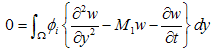 | (31) |
where φi is the test function and Ω is the region of the flow.Consider a two parameter (semi-discrete) Galerkin approximation[10,11] of the form: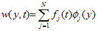 | (32) |
with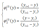 | (33) |
where i=1,2,3,…..,N and yi and yi+1 are respectively the lower and upper coordinates of the element i.Using Equations (32-33), Equation (31) reduces to: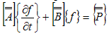 | (34) |
where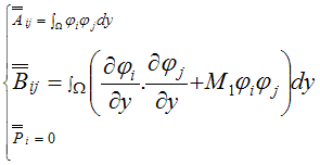 | (35) |
Using the Θ - family of operators developed by Reddy [11], Equation (34) takes the form: | (36) |
where | (37) |
The numerical values of the temperature and velocity fields have been computed from Equations (23), (29) and (36) and are shown in Figures.2-5.
3. Discussion of Results
To study the behavior of the velocity and temperature profiles, curves are drawn for various values of the parameters that describe the flow. Numerical calculations have been carried out for the velocity and temperature distributions for m=0 and λ=1, reducing M1 to M2. The results obtained are displayed in Figures 2-5. The method used is unconditionnaly stable and independent of the time step Δt. The velocity profiles are examined for the cases Gr > 0 and Gr < 0. Gr > 0 (= +5) is used for the case when the flow is in the presence of cooling of the plate by free convection currents. Gr < 0 (= -5) is used for the case when the flow is in the presence of heating of the plate by free convection currents. Figures 2-4 show the velocity distribution for the two cases from which we observe that the velocity (u) decreases away from the plate.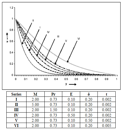 | Figure 2. Primary velocity (u) distribution for Gr = 5. |
From Figure 2, for the case when Gr>0 (in the presence of cooling of the plate by free convection currents), we observe that:i. The primary velocity (u) decreases due to an increase in the magnetic parameter M.ii. The primary velocity (u) increases due to an increase in the Prandtl number Pr, the Eckert number E, the heat source parameter δ and the time t.From Figure 3, for the case when Gr<0 (in the presence of heating of the plate by free convection currents), we observe that:i. The primary velocity (u) decreases due to an increase in the magnetic parameter M, the Prandtl number Pr, the Eckert number E and the heat source parameter δ.ii. The primary velocity (u) increases due to an increase in the time t.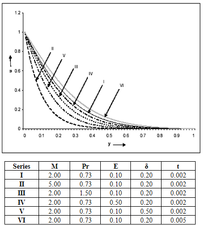 | Figure 3. Primary velocity (u) distribution for Gr = -5. |
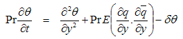
From Figure 4, for the case when Gr = ±5, we observe that:i. The secondary velocity (w) decreases due to an increase in the magnetic parameter M and the time parameter t. ii. There is an insignificant change in the secondary velocity (w) due to an increase in the Prandtl number Pr, the Eckert number E and the heat source parameter δ.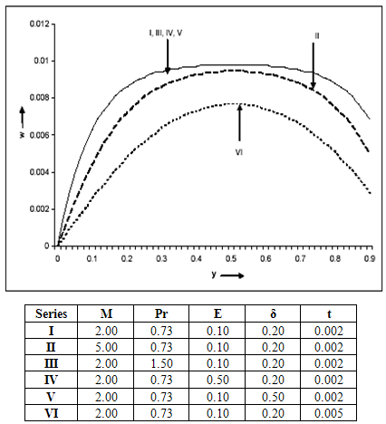 | Figure 4. Secondary velocity (w) distribution for Gr = ±5 |
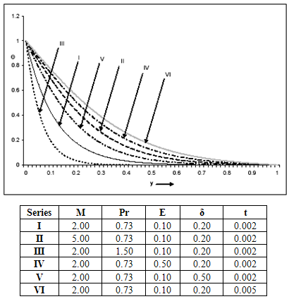 | Figure 5. Temperature (Ө) distribution for Gr = ±5. |
From Figure 5, for the case when Gr = ±5, we observe that:i. The temperature (Ө) decreases far away from the plate. The decrease is greater for a Newtonian fluid than it is for a non-Newtonian fluid (Ө decreases with Pr). ii. There is an increase in the temperature profile (Ө) due to an increase in the magnetic parameter M, the Eckert number E, the heat source parameter δ and the time parameter t.
Nomenclature
g : the gravitational accelerationβ : the volumetric coefficient of thermal expansionv : the kinematic coefficient of viscosity of the fluidk : the thermal conductivityρ : the density of the fluidQ* : the heat generation of the type Cp : the specific heat at constant pressureT/ : the temperature in the boundary layer : the temperature in the free streamPr : the Prandtl numberGr : the Grashof numberM2 : the magnetic field parameterδ : the heat source parameterσ: the electric conductivityμe: the magnetic permeabilityωe: the cyclotron frequencyτe: the electron collision timee: the electric chargene : the number density of electronsPe : the electron pressureQ: the velocity of the fluidu: the non-dimensional primary velocityw: the non-dimensional secondary velocityӨ: the non-dimensional temperature
References
| [1] | Rossow VJ. On the flow of electrically conducting fluid over a flat plate in the presence of transverse magnetic field. NASA Report 1958; 1358 |
| [2] | Soundalgekar VM, Gupta SK, Aranake RN. Free convection effects on MHD Stokes problem for a vertical plate. Nuclear Engineering and Design. 1978; 51: 403-407 |
| [3] | Pop I. The effects of Hall currents on hydromagnetic flow near an accelerated plate. J. Math. And Phys. Sci. 1971; 5: 375-386 |
| [4] | Naroua, H. A computational solution of hydromagnetic-free convective flow past a vertical plate in a rotating heat-generating fluid with Hall and ion-slip currents, International Journal for Numerical Methods in Fluids 2007; 53: 1647-1658 |
| [5] | Khan M, Maqbool K and Hayat T. Influence of Hall current on the flows of a generalized Oldroyd-B fluid in a porous space. Acta Mechanica 2006; 184(1-4): 1-13 |
| [6] | Kinyanjui M, Kwanza JK and Uppal SM. Magnetohydrodynamic free convection heat and mass transfer of a heat generating fluid past an impulsively started infinite vertical porous plate with Hall current and radiation absorption. Energy conversion and management 2001; 42(8): 917-931 |
| [7] | Ram PC. Hall effects on hydromagnetic free convective flow and mass transfer through a porous medium bounded by an infinite vertical porous plate with constant heat flux. International Journal of Energy Research 1988; 12: 227-231 |
| [8] | Shercliff JA. A Text Book of Magnetohydrodynamics. Pergamon Press, New York (USA). 1975 |
| [9] | Cowling TG. Magnetohydrodynamics. Interscience, New York (USA). 1957 |
| [10] | Naroua H, Takhar HS, Slaouti A. Computational challenges in fluid flow problems: a MHD Stokes problem of convective flow from a vertical infinite plate in a rotating fluid. European Journal of Scientific Research 2006; 13 (1): 101-112 |
| [11] | Reddy JN. An Introduction to the finite element method. Mc Graw Hill book company: Singapore 1984 |
 Abstract
 Reference
 Full-Text PDF
 Full-Text HTML