Stefanos Drakos
International Centre of Computational Engineering, Rhodes, Greece
Correspondence to: Stefanos Drakos, International Centre of Computational Engineering, Rhodes, Greece.
| Email: |  |
Copyright © 2016 Scientific & Academic Publishing. All Rights Reserved.
This work is licensed under the Creative Commons Attribution International License (CC BY).
http://creativecommons.org/licenses/by/4.0/

Abstract
The Growth of Cancer Tumor study is one of the most critical problems in the modern society. Million of deaths are recorded every day because of disease. The calculation of the growth has been addressed in the past by many scientists and is a very important factor for the correct strategy of treatment during the period of therapies. The knowledge of the tumor growth probability at each time is an important quantity for the problem definition. A Fokker Plank equation of a stochastic Gompertz law of growth was set up and a finite element based model solved the evolution of transition density function. In a numerical example at the end, the effect of the therapy and the width of fluctuation in the probability history are investigated.
Keywords:
Stochastic Growth of Cancer Tumor, Fokker Plank equation, Finite Element Method
Cite this paper: Stefanos Drakos, On Stochastic Model for the Growth of Cancer Tumor based on the Finite Element Method, American Journal of Biomedical Engineering, Vol. 6 No. 6, 2016, pp. 166-169. doi: 10.5923/j.ajbe.20160606.02.
1. Introduction
The growth of cancer tumor modeling was the subject of research for many years. The majority of the models were based on the deterministic Gompertz law of growth, but which cannot capture the uncertainties of the phenomenon thus not realistic. To overcome this weakness various mathematical models considering the problem as stochastic rather as deterministic were developed the last years. In [1] the probability of tumor extinction due to the action of cytotoxic cell populations was investigated by several one dimensional stochastic models of the population growth and elimination processes of a tumor. In [2] A stochastic model was proposed to study the problem of inherent resistance by cell populations when chemotherapeutic agents are used to control tumor growth. Stochastic differential equations were introduced and numerically integrated to simulate expected response to the chemotherapeutic strategies as a function of different parameters. A stochastic model of solid tumor growth based on deterministic Gompertz law was presented in [5]. The proposed model was also implemented to simulate the effects of a time-dependent therapy. In [6] a stochastic model in tumour growth, based upon the deterministic Gompertz law of cell growth was proposed. This model took account of both cell fission and mortality too. The corresponding density function of the size of the tumour cells obeys a functional Fokker--Planck equation which can be solved analytically. A new Gompertz-type diffusion process was is introduced in [7], by means of which bounded sigmoidal growth patterns can be modeled by time-continuous variables. The main innovation of the process was that the bound can depend on the initial value. In [8] Based upon the deterministic Gompertz law of cell growth, a stochastic model of tumour cell growth were proposed, in which the size of the tumour cells is bounded. The model takes account of both cell fission (which is an ‘action at a distance’ effect) and mortality too. Accordingly, the density function of the size of the tumour cells obeys a functional Fokker–Planck Equation (FPE) associated with the bounded stochastic process. In [9] a Gompertz-type diffusion process, which includes in the drift term a time-dependent function C(t) representing the effect of a therapy able to modify the dynamics of the underlying process was developed. So a statistical approach was proposed in order to estimate this function when a control group and one or more treated groups are observed. In [10] a diffusion model based on a generalized Gompertz deterministic growth in which carrying capacity depends on the initial size of the population was considered. The drift of the resulting process is then modified by introducing a time-dependent function, called "therapy", in order to model the effect of an exogenous factor. The transition probability density function and the related moments for the proposed process were obtained. In [11] a Gompertz-type diffusion process characterized by the presence of exogenous factors in the drift term was considered. This process is able to describe the dynamics of populations in which both the intrinsic rates are modified by means of time-dependent terms. The understanding and the assessment of the tumor growth is a very critical subject that results in the selection of successful treatment strategy [3, 4]. In this paper, taking into account the stochastic process based on the deterministic Gompertz law as presented in [9] and introducing the methods of engineering such as the finite element method, the problem of the transition probability density evolution was solved. Knowing each time the value of this quantity the probability of the tumor growth can be calculated.
2. The Stochastic Model
Suppose  is a probability space with a filtration
  . Where
  is the σ- algebra and is considered to contain all the information that is available,
  is the probability measure. According the work of [9] the growth of cancer tumor assuming that follows the stochastic process
  :
: | (1) |
Where α, b and σ are positive constants representing the growth, death rates and the width of random fluctuations, respectively, and W(t) is a standard Brownian motion. The function C(t) represent the effect of the therapy and can be considering as constant or as time depended. For  given the transition probability density
  we can estimate at each time t the probability that the process X(t) takes a specific value. The transition probability density
  with normalization condition:
 | (2) |
 | (3) |
Where δ is the Dirac Delta functionAnd  | (4) |
The transition probability density  obeys the Fokker–Planck equation and can be given by the equation:
 | (5) |
To solve this equation a transformation must be carried out before. Suppose a function  of
of  class in t and
  class in x and
  where
where 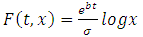 | (6) |
By Ito formula we get: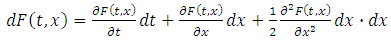 | (7) |
Where: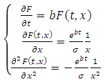 | (8) |
Substituting the resultant derivatives of 8 in 7: 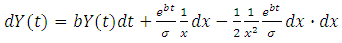 | (9) |
From equation 5 and 9 we get: | (10) |
And finally: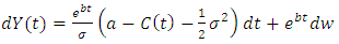 | (11) |
The Fokker–Planck equation in the new form according to the process of equation 11 is given as: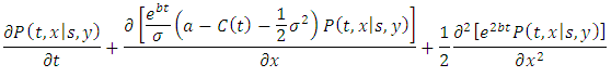 | (12) |
Or: | (13) |
The infinitesimal generator for this process has constant coefficients: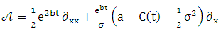 | (14) |
3. Finite Element Method for Fokker-Planck Equation
Finite element method has been used in many areas of engineering in last decades. The method gains a great interest of application in the area of stochastic problems and in the quantification of uncertainty during the past years. Different problems of uncertainty’s quantification has been solved in the geomechanics [12] and in financial engineering [13] fields by the author. The successful widely used of the finite element method in order to investigate the evolution of the probability density function of linear and nonlinear 2d and 3d problems in dynamics engineering attract our interest for the numerical solution of Fokker Planck equation [14, 15]. The stability and the generality are some of the advantages among others of the method for the time dependent problems. In order to solve the problem in equation 17 according to the finite element method in the current paper we consider a linear element with nodes 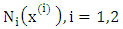 . To each node
  there is a hat function
  . Let
. Let 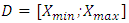 the domain which is an interval on the real axis with the
  are referring to the boundaries of tumor growth and the
  on the tumor capacity. By subdividing the initial domain into smaller subintervals we can get the probability density function within the
  subinterval interpolated by the hat functions:
 | (15) |
Where φm are the hat functions, M is the number of node at each element and  is probability density function at each node. To solve the problem assuming a test
  function belongs to the space:
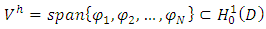 | (16) |
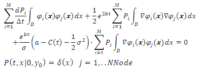
For every test function  and integrating by parts over the domain D the variational formulation of the Cancer Tumor probability transition density equation has the following form:
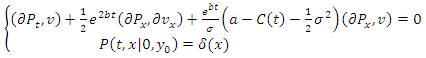 | (17) |
Where δ is the Dirac Delta functionThe equation 17 can be written as: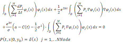 | (18) |
 | (19) |
Using the matrix notation the equation 19 takes the following form: 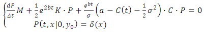 | (20) |
Where: 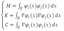 | (21) |
3.1. Time Discretization
According to the previous replacement we discretize the equation 20 using the theta-scheme with constant time step Δt. The finite element mesh considered as uniform and the equation 20 takes the following form: 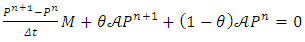 | (22) |
Equivalent | (23) |
These equations consist of a system of linear algebraic equations which must be solved at each time step to advance the numerical solution for the density function. The verification of the algorithm and the accuracy of the method was presented by author in the form of Black-Sholes in [13]. A numerical example has been solved in order to investigate the results of fluctuation and the therapy effects on the history of probability density function are presented in the following example. Assuming for the growth and death rate a=0.5 and b=0.1 respectively. Four different cases was solved for the effect of therapy on the tumor growth. In the first an untreated case was carried out and then three more with constant value of 0.1, 0.2, and 0.3. For each case of therapy the effect of four different values of fluctuation taken to account 0.1, 0.2, 0.3, 0.4. The evolution of probability density for the various cases in the following pictures are presented. The problem was solved for three different time of t=2, 4, 8 and as its cleared the effect of therapy in the figure 1 while as the fluctuation increase the effect has opposite result in the history of the transition density.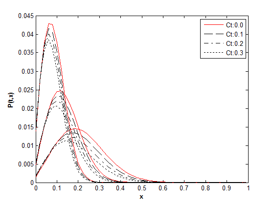 | Figure 1. Τime history of transition density function for σ=0.1 |
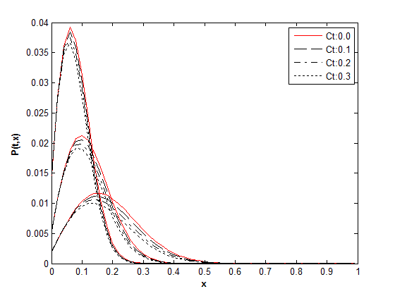 | Figure 2. Τime history of transition density function for σ=0.2 |
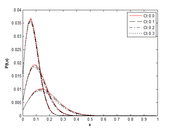
 | Figure 3. Τime history of transition density function for σ=0.3 |
 | Figure 4. Τime history of transition density function for σ=0.4 |
4. Application of the Model
In practice the model can be used to estimate the appropriate dose of therapy based on the probability of the tumor growth.At each time for a given size of tumor and knowing the effect of the therapy the probability for a future size of tumor can be evaluated. This gives us the effort to update at each time the level of therapy. Thus for a given size of tumor x at time  the probability of reaching a specific size y can be given by the following equation:
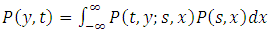 | (24) |
5. Conclusions
Fokker Planck equation was set up in order to calculate the evolution of the probability density function of the Cancer Tumor Growth. The process are based on the Gompertz law of growth and taken into the account the effect of therapy. A finite element method was used to solve the time dependent problem of the probability evolution. A numerical example solved at the end and the effect of the therapy and the width of the fluctuation are investigated on the probability history of the tumor growth.
References
| [1] | Merrill SJ. Stochastic models of tumor growth and the probability of elimination by cytotoxic cells, J Math Biol. 1984; 20(3): 305-20. |
| [2] | Abundo M, Rossi C. Numerical simulation of a stochastic model for cancerous cells submitted to chemotherapy J Math Biol. 1989; 27(1): 81-90. |
| [3] | L. Ferrante, S. Bompadre, L. Possati, and L. Leone, Parameter estimation in a Gompertzian stochastic model for tumor growth, Biometrics 56 (2000), p. 1076. |
| [4] | C. Guiot, P.G. Degiorgis, P.P. Delsanto, P. Gabriele, and T.S. Deisboeck, Does tumor growth follow a universal law, J. Theor. Biol. 225 (2003), p. 147. |
| [5] | Albano G, Giorno V. A stochastic model in tumor growth. J Theor Biol. 2006 Sep 21; 242(2):329-36. Epub 2006 Apr 19. |
| [6] | C. F. Lo Stochastic Gompertz model of tumour cell growth. J Theor Biol. 2007 Sep 21; 248(2): 317–321. |
| [7] | Gutiérrez-Jáimez R, Román P, Romero D, Serrano JJ, Torres F. A new Gompertz-type diffusion process with application to random growth, Math Biosci. 2007 Jul; 208(1): 147-65. Epub 2006 Oct 14. |
| [8] | C. F. Lo, A modified stochastic Gompertz model for tumour cell growth, Computational and Mathematical Methods in Medicine Vol. 11, No. 1, March 2010, 3–11. |
| [9] | Albano G, Giorno V, Román-Román P, Torres-Ruiz F. Inferring the effect of therapy on tumors showing stochastic Gompertzian growth, J Theor Biol. 2011 May 7; 276(1): 67-77. doi: 10.1016/j.jtbi.2011.01.040. Epub 2011 Feb 3. |
| [10] | Albano G, Giorno V, Román-Román P, Torres-Ruiz F., On the therapy effect for a stochastic growth Gompertz-type model Math Biosci. 2012 Feb; 235(2): 148-60. doi: 10.1016/j.mbs.2011.11.007. Epub 2011 Nov 28. |
| [11] | Albano G, Giorno V, Román-Román P, Torres-Ruiz F., On the effect of a therapy able to modify both the growth rates in a Gompertz stochastic model, Math Biosci. 2013 Sep; 245(1): 12-21. doi: 10.1016/j.mbs.2013.01.001. Epub 2013 Jan 21. |
| [12] | Stefanos Drakos, Quantitative of uncertainty in unconfined flow problems, International Journal of Geotechnical Engineering Volume 10, 2016 - Issue 3. |
| [13] | Drakos, S. Uncertain Volatility Derivative Model Based on the Polynomial Chaos. Journal of Mathematical Finance, 6, 55-63. doi: 10.4236/jmf.2016.61007. (2016). |
| [14] | B.F. Spencer and L.A. Bergman. On the numerical solutions of the Fokker-Planck equations for nonlinear stochastic systems. Nonlinear Dynamics, 4:357–372, 1993. |
| [15] | P. Kumar and S. Narayana. Solution of Fokker-Planck equation by finite element and finite difference methods for nonlinear systems. Sadhana, 31-4:445–461, 2006. |

 Abstract
 Reference
 Full-Text PDF
 Full-text HTML